ggplot(fatal_crash_smry_by_state)
ggplot(fatal_crash_smry_by_state) + aes(x = death_rate_vmt, y = state)
ggplot(fatal_crash_smry_by_state) + aes(x = death_rate_vmt, y = state) + geom_point()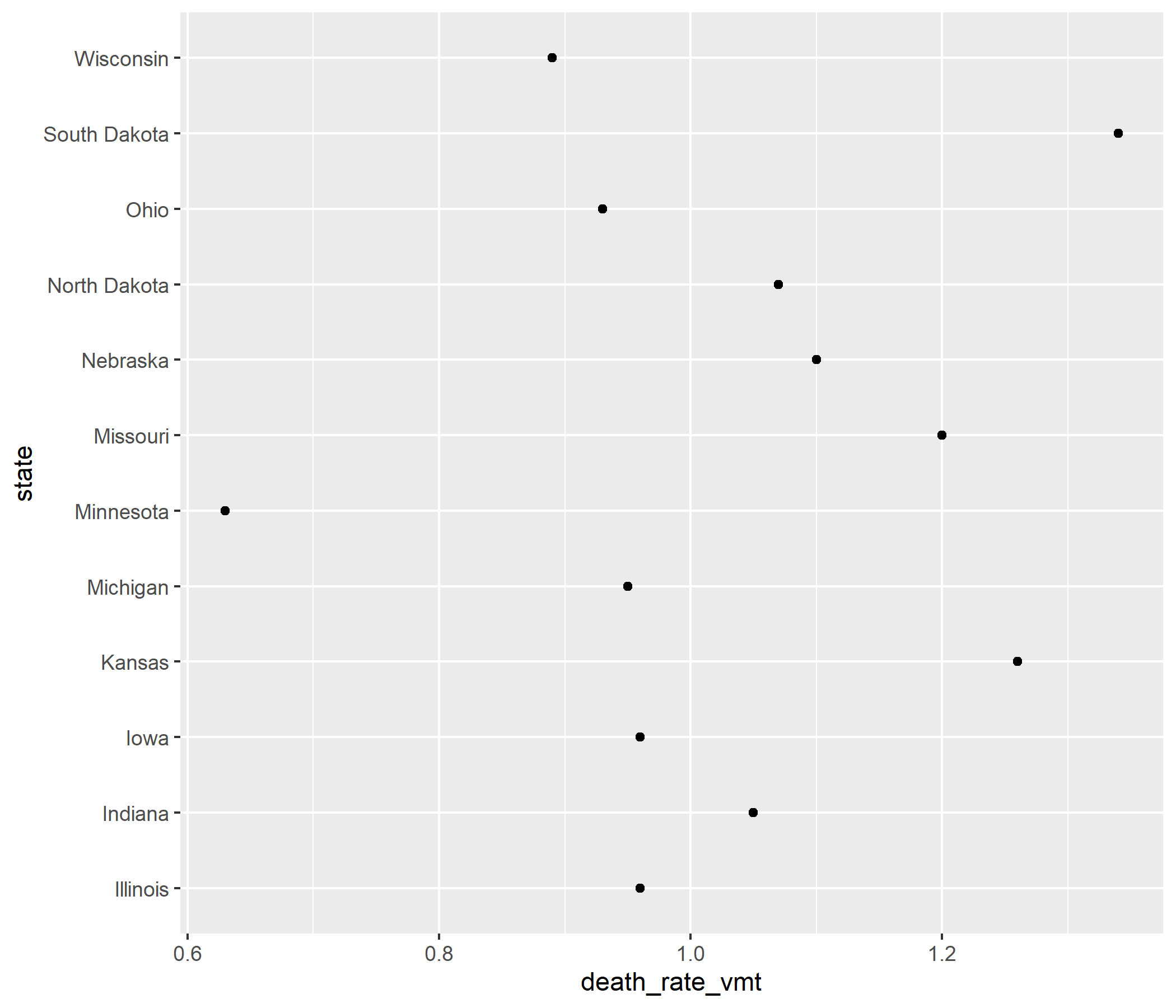
ggplot(fatal_crash_smry_by_state) + aes(x = death_rate_vmt, y = state) + geom_point() + aes( y = fct_reorder( state, death_rate_vmt ) )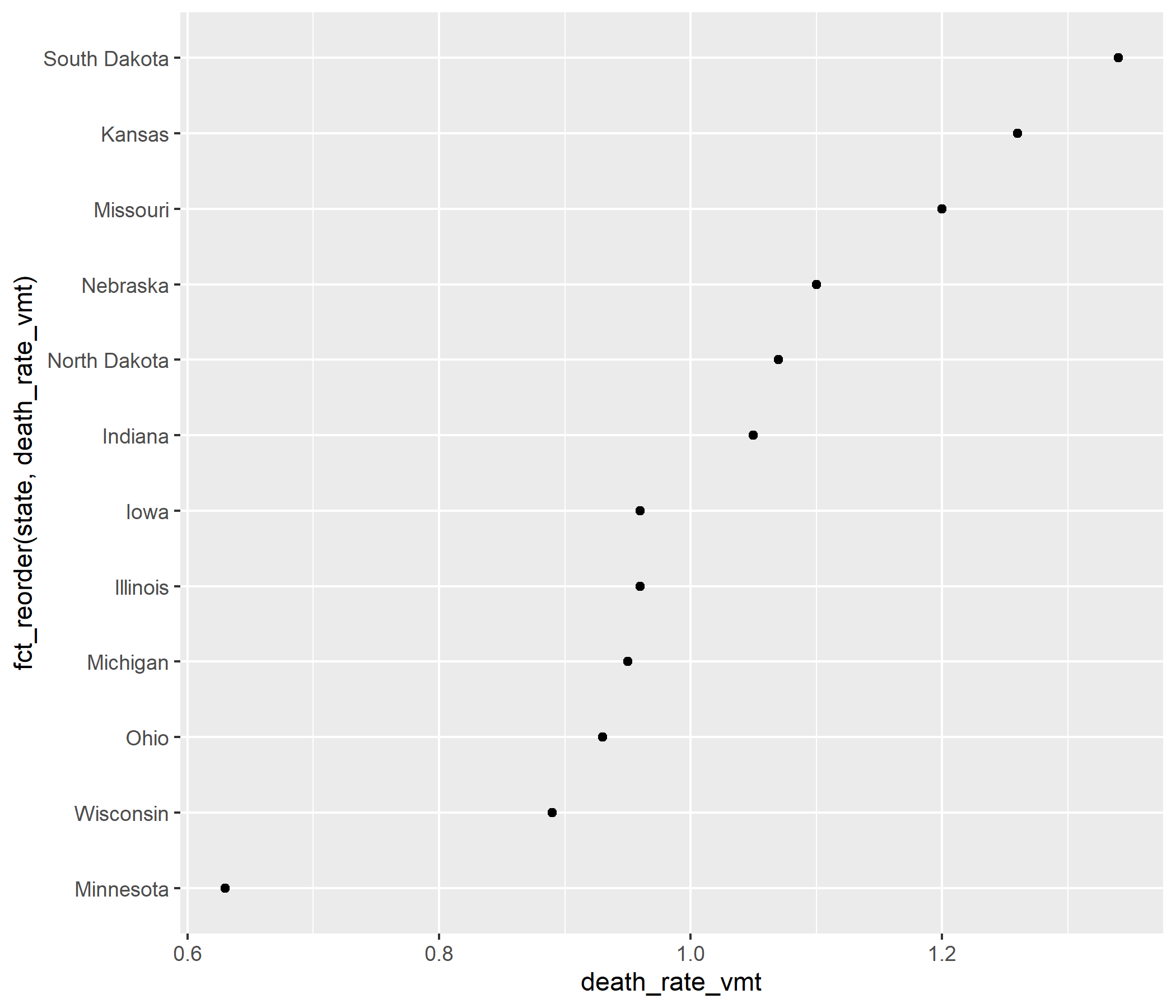
ggplot(fatal_crash_smry_by_state) + aes(x = death_rate_vmt, y = state) + geom_point() + aes( y = fct_reorder( state, death_rate_vmt ) ) + geom_segment( aes( x = 0, y = state, xend = death_rate_vmt, yend = state ) )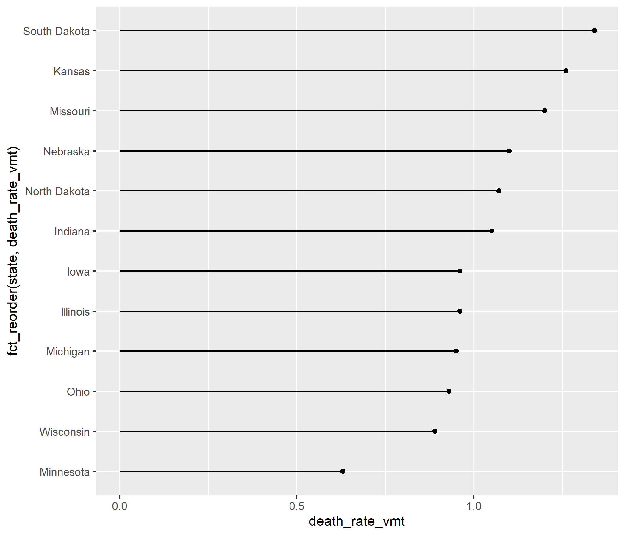
ggplot(fatal_crash_smry_by_state) + aes(x = death_rate_vmt, y = state) + geom_point() + aes( y = fct_reorder( state, death_rate_vmt ) ) + geom_segment( aes( x = 0, y = state, xend = death_rate_vmt, yend = state ) ) + labs( x = paste( "Deaths per 100 million", "vehicle miles traveled" ) )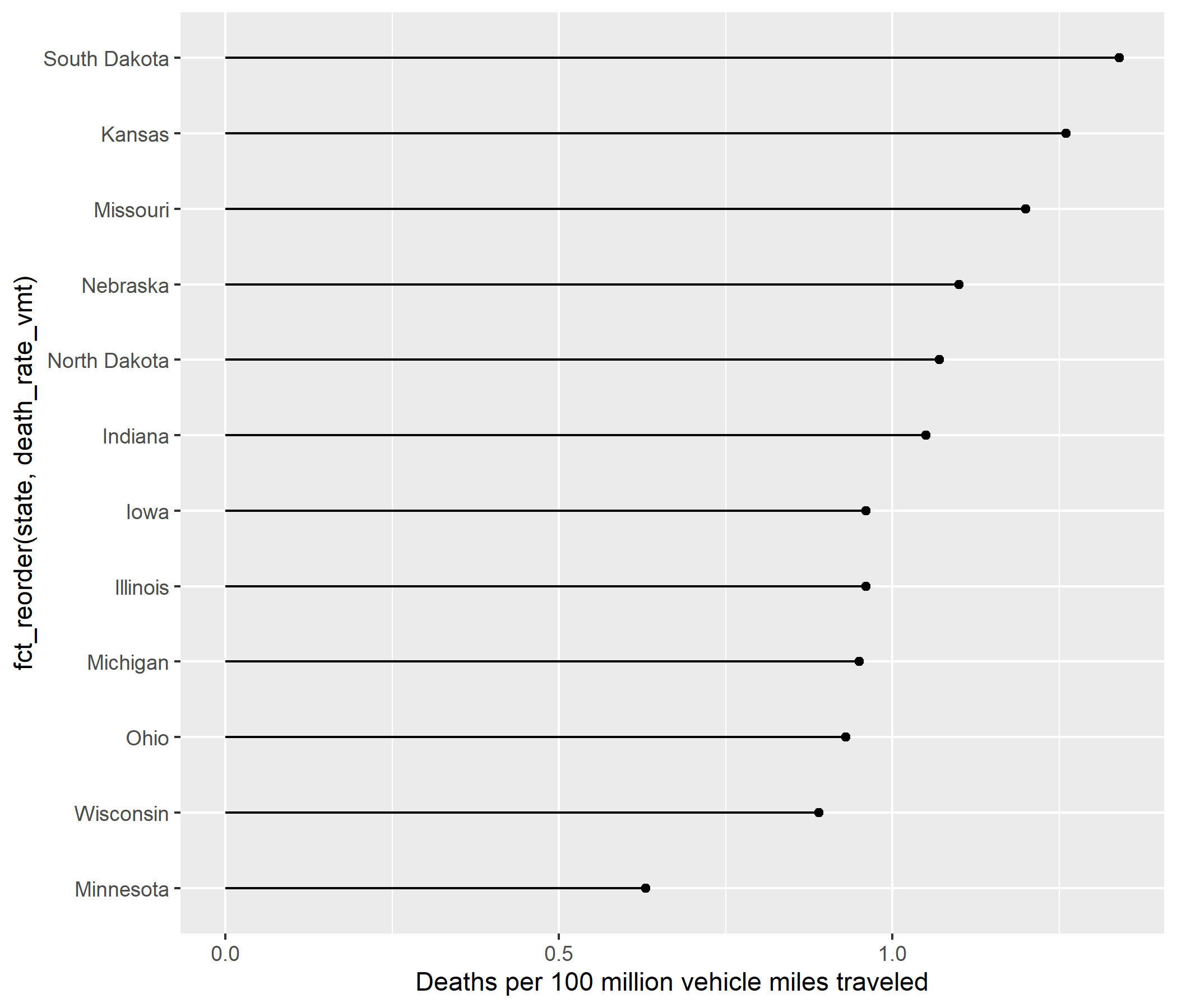
ggplot(fatal_crash_smry_by_state) + aes(x = death_rate_vmt, y = state) + geom_point() + aes( y = fct_reorder( state, death_rate_vmt ) ) + geom_segment( aes( x = 0, y = state, xend = death_rate_vmt, yend = state ) ) + labs( x = paste( "Deaths per 100 million", "vehicle miles traveled" ) ) + labs(y = "Midwestern state")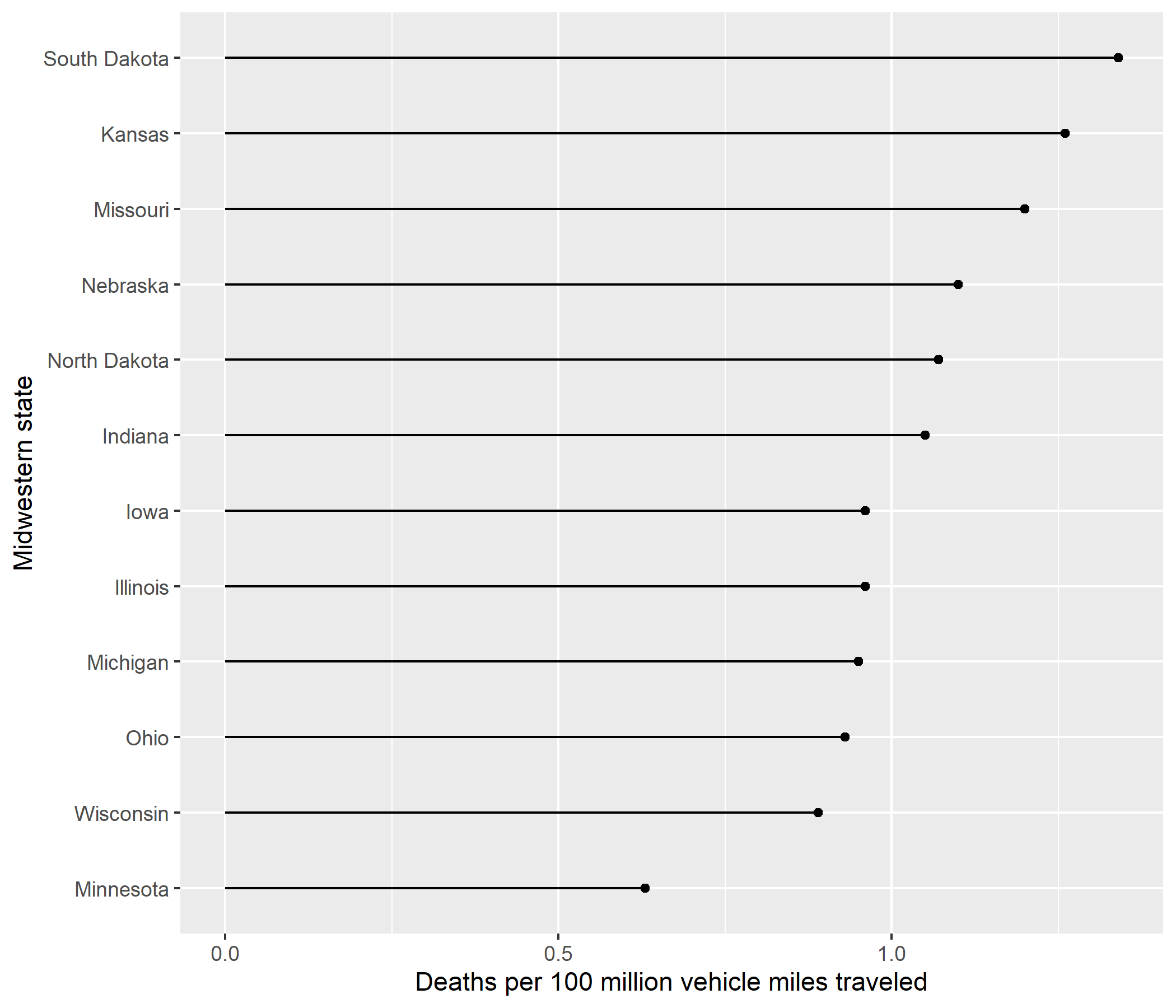
ggplot(fatal_crash_smry_by_state) + aes(x = death_rate_vmt, y = state) + geom_point() + aes( y = fct_reorder( state, death_rate_vmt ) ) + geom_segment( aes( x = 0, y = state, xend = death_rate_vmt, yend = state ) ) + labs( x = paste( "Deaths per 100 million", "vehicle miles traveled" ) ) + labs(y = "Midwestern state") + labs( title = paste( "Motor vehicle crash death rate", "per midwestern state, 2018" ) )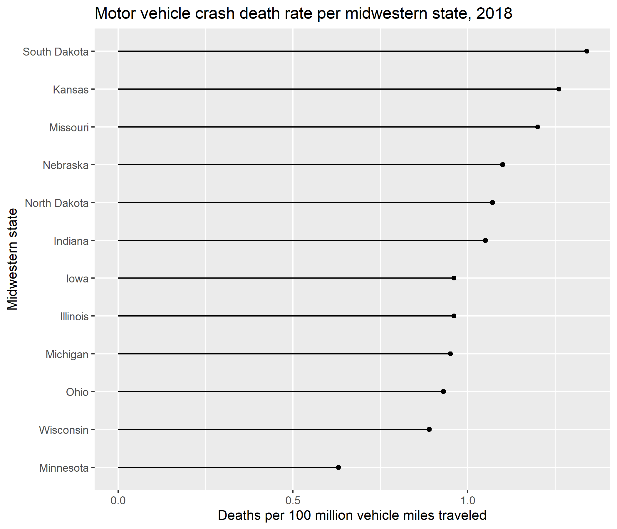
ggplot(fatal_crash_smry_by_state) + aes(x = death_rate_vmt, y = state) + geom_point() + aes( y = fct_reorder( state, death_rate_vmt ) ) + geom_segment( aes( x = 0, y = state, xend = death_rate_vmt, yend = state ) ) + labs( x = paste( "Deaths per 100 million", "vehicle miles traveled" ) ) + labs(y = "Midwestern state") + labs( title = paste( "Motor vehicle crash death rate", "per midwestern state, 2018" ) ) + labs(caption = "Data source: IIHS")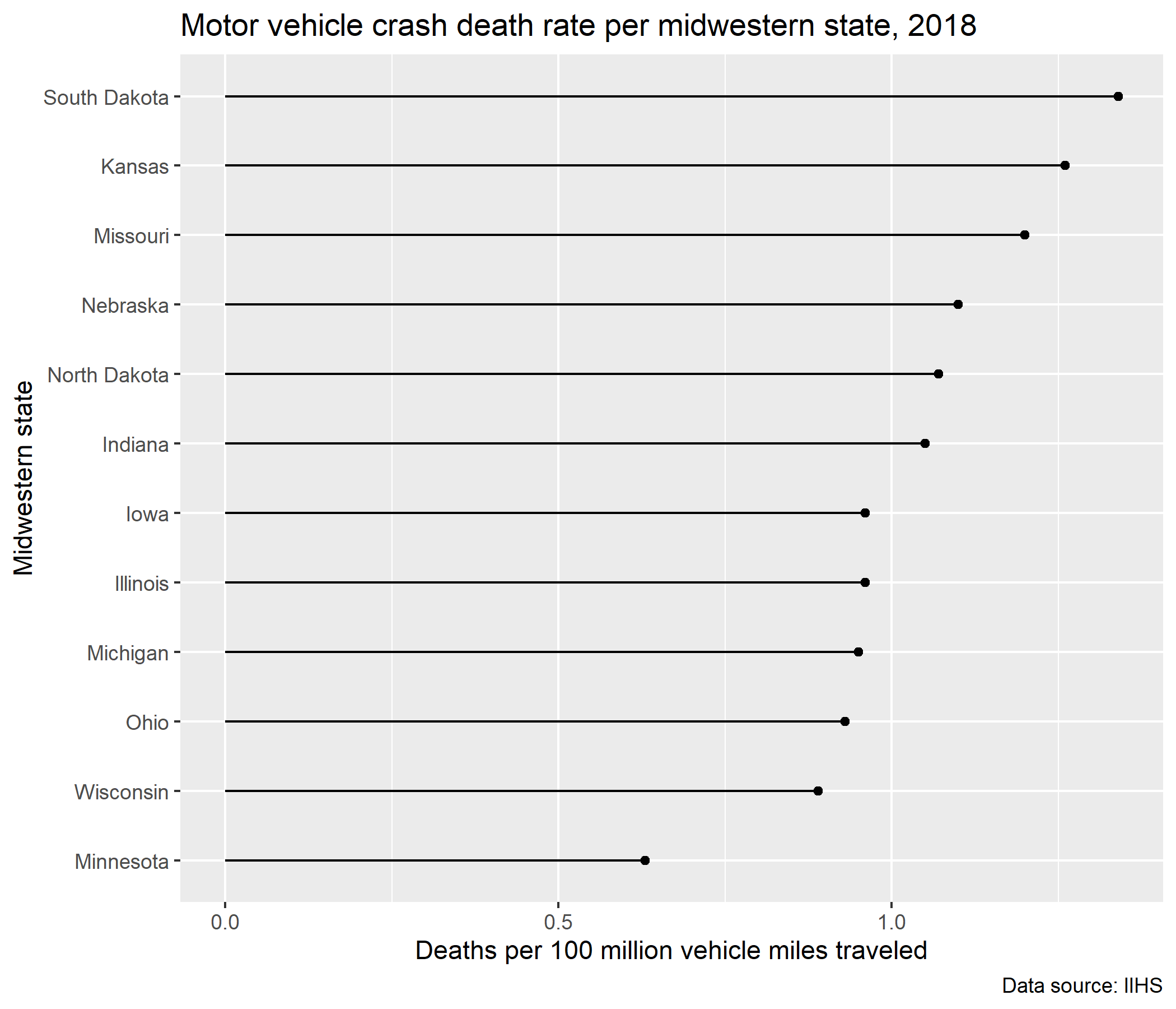
ggplot(fatal_crash_smry_by_state) + aes(x = death_rate_vmt, y = state) + geom_point() + aes( y = fct_reorder( state, death_rate_vmt ) ) + geom_segment( aes( x = 0, y = state, xend = death_rate_vmt, yend = state ) ) + labs( x = paste( "Deaths per 100 million", "vehicle miles traveled" ) ) + labs(y = "Midwestern state") + labs( title = paste( "Motor vehicle crash death rate", "per midwestern state, 2018" ) ) + labs(caption = "Data source: IIHS") + gghighlight(state == "Iowa")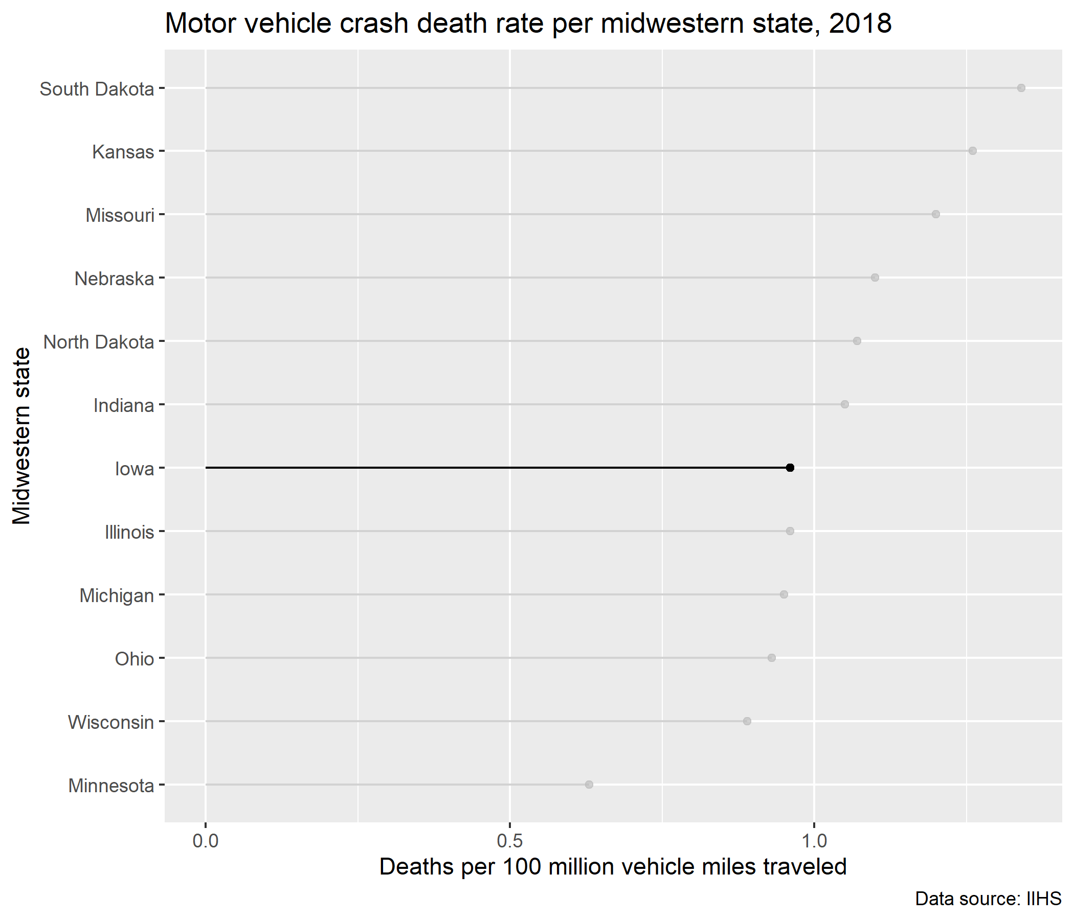
ggplot(fatal_crash_monthly_counts)
ggplot(fatal_crash_monthly_counts) + aes( x = crash_month, y = fatal_crash_freq )
ggplot(fatal_crash_monthly_counts) + aes( x = crash_month, y = fatal_crash_freq ) + aes(group = crash_year)
ggplot(fatal_crash_monthly_counts) + aes( x = crash_month, y = fatal_crash_freq ) + aes(group = crash_year) + geom_line()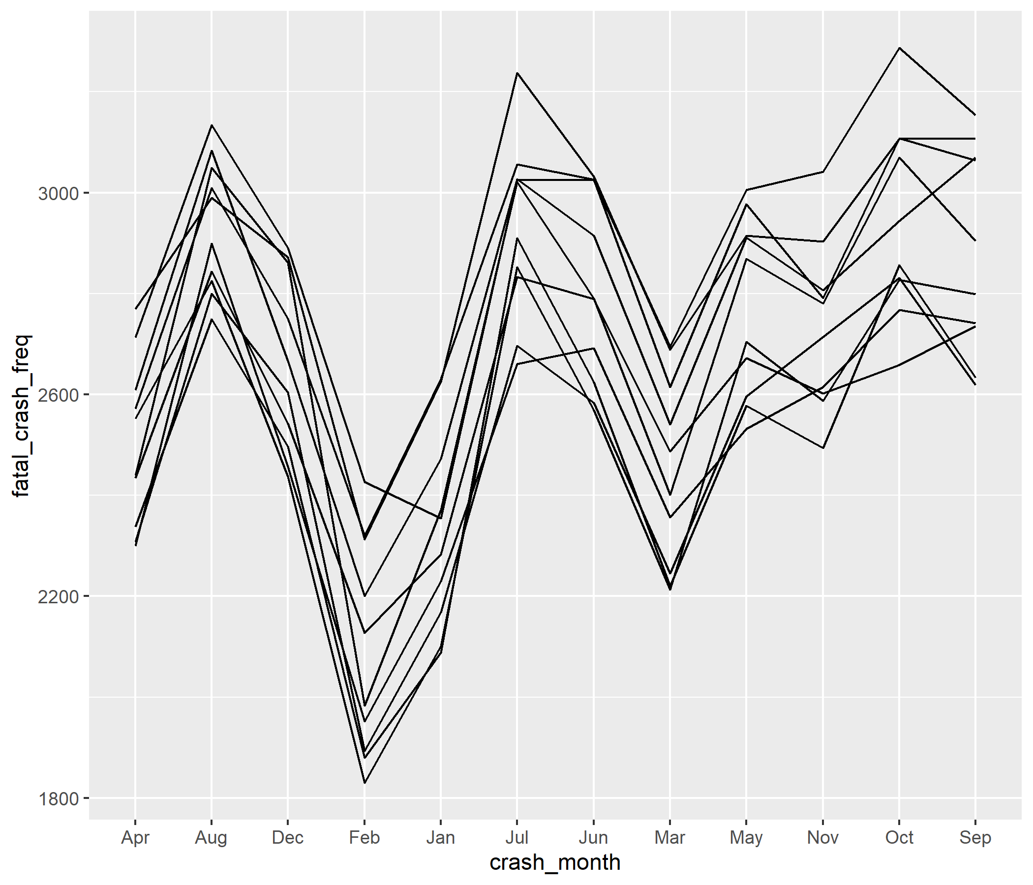
ggplot(fatal_crash_monthly_counts) + aes( x = crash_month, y = fatal_crash_freq ) + aes(group = crash_year) + geom_line() + scale_x_discrete(limits = month.abb)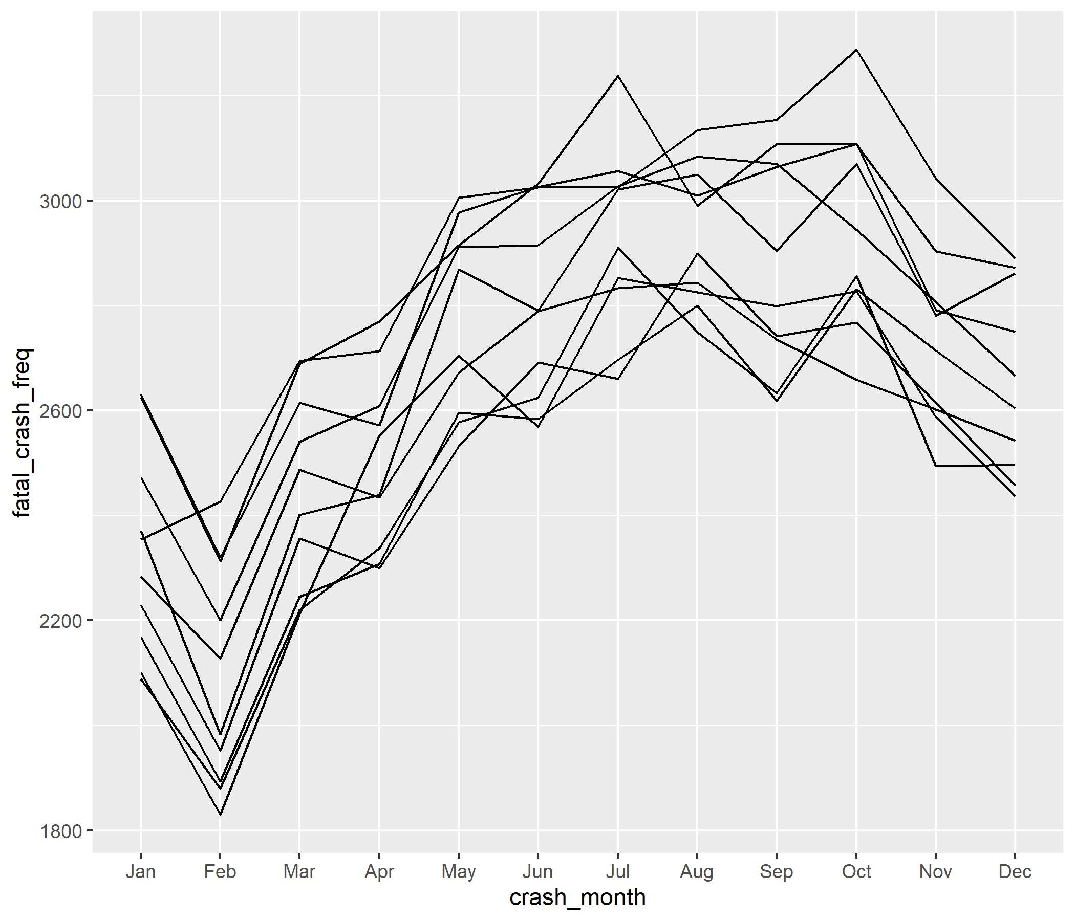
ggplot(fatal_crash_monthly_counts) + aes( x = crash_month, y = fatal_crash_freq ) + aes(group = crash_year) + geom_line() + scale_x_discrete(limits = month.abb) + aes(color = factor(crash_year))
ggplot(fatal_crash_monthly_counts) + aes( x = crash_month, y = fatal_crash_freq ) + aes(group = crash_year) + geom_line() + scale_x_discrete(limits = month.abb) + aes(color = factor(crash_year)) + labs(x = "Crash month")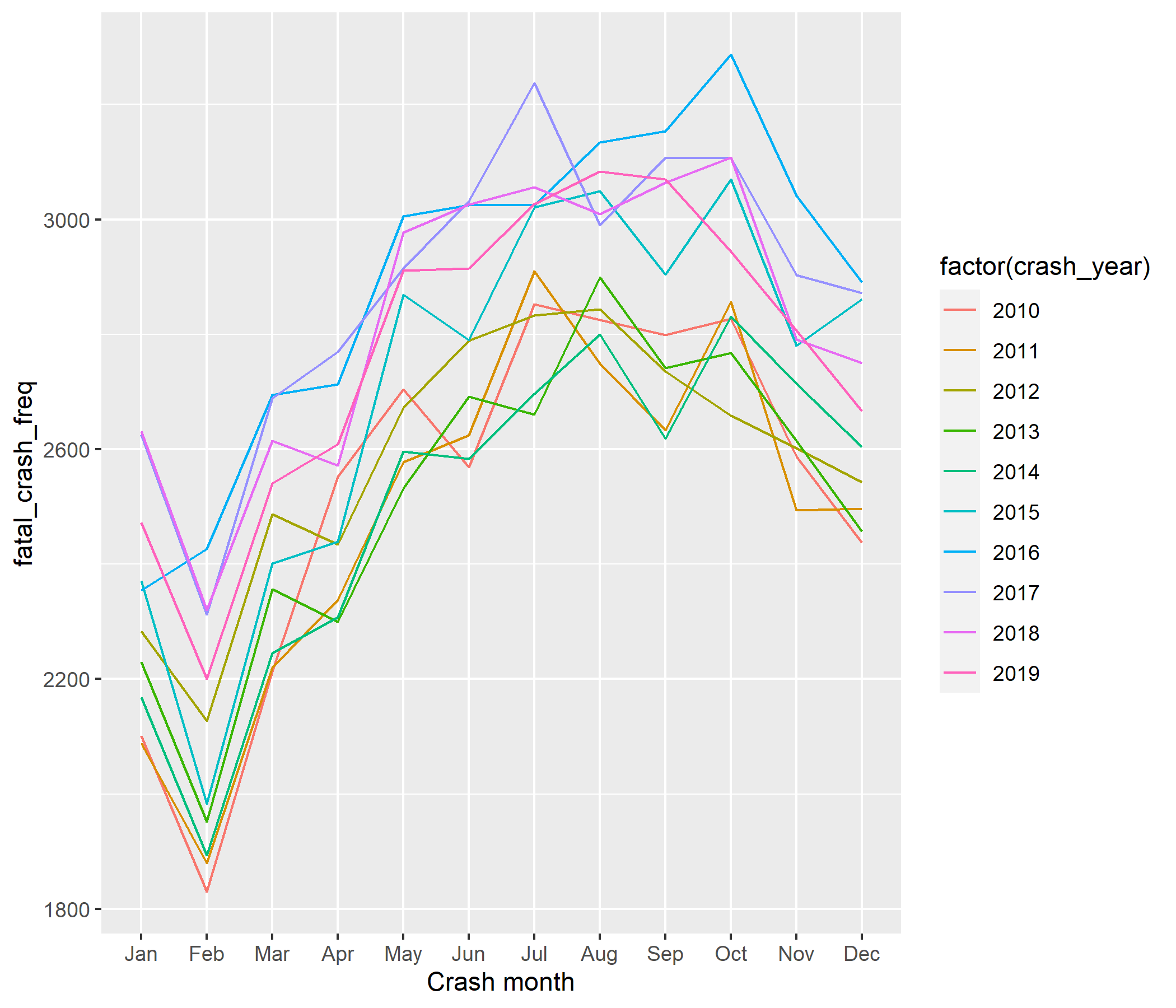
ggplot(fatal_crash_monthly_counts) + aes( x = crash_month, y = fatal_crash_freq ) + aes(group = crash_year) + geom_line() + scale_x_discrete(limits = month.abb) + aes(color = factor(crash_year)) + labs(x = "Crash month") + labs(y = "Fatal crash frequency")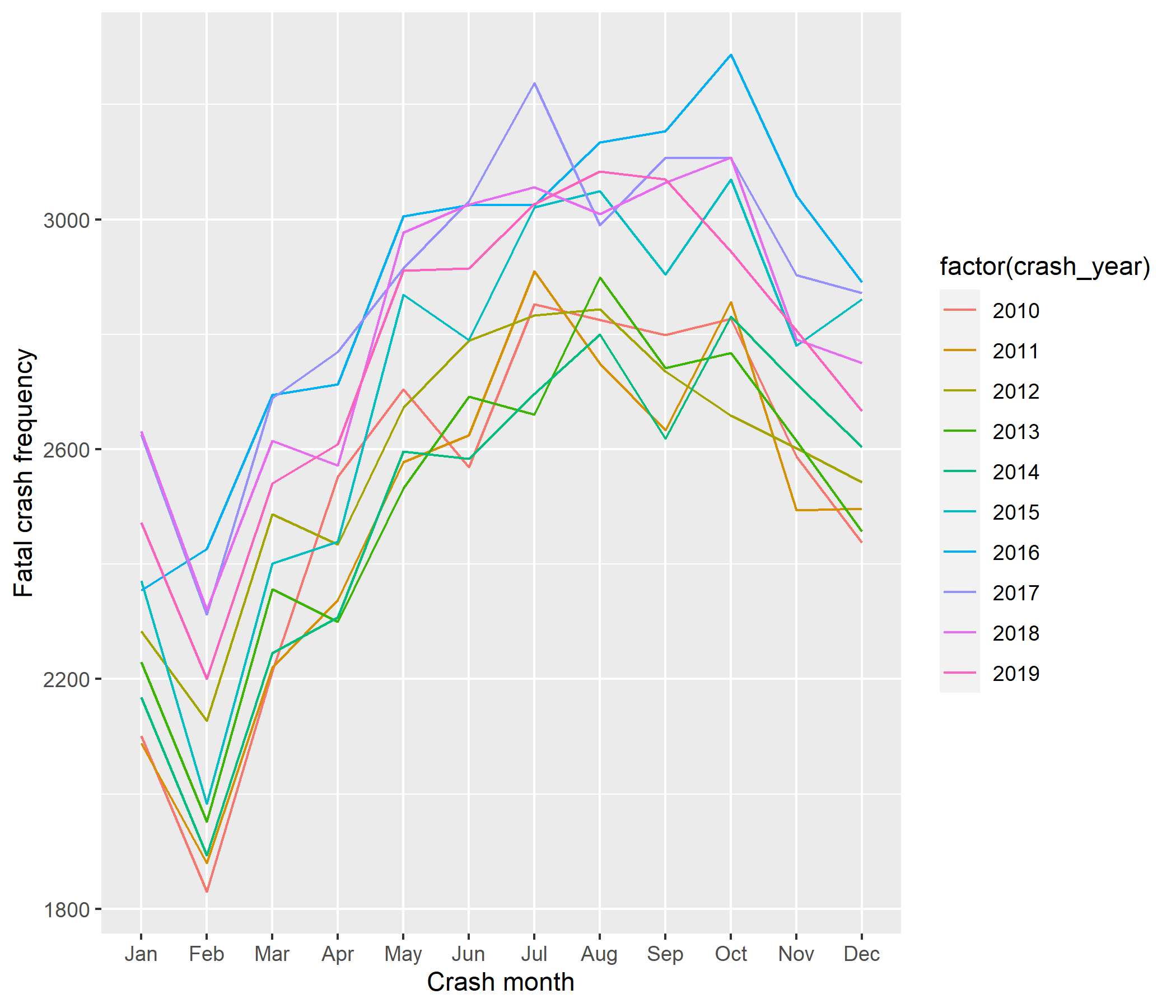
ggplot(fatal_crash_monthly_counts) + aes( x = crash_month, y = fatal_crash_freq ) + aes(group = crash_year) + geom_line() + scale_x_discrete(limits = month.abb) + aes(color = factor(crash_year)) + labs(x = "Crash month") + labs(y = "Fatal crash frequency") + labs(color = "Crash year")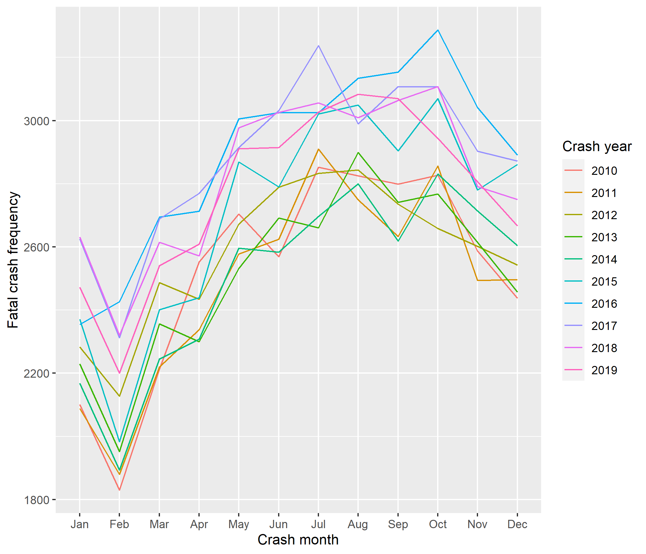
ggplot(fatal_crash_monthly_counts) + aes( x = crash_month, y = fatal_crash_freq ) + aes(group = crash_year) + geom_line() + scale_x_discrete(limits = month.abb) + aes(color = factor(crash_year)) + labs(x = "Crash month") + labs(y = "Fatal crash frequency") + labs(color = "Crash year") + labs( title = paste( "Motor vehicle fatal crash trend", "in the U.S. by month, 2010–2019" ) )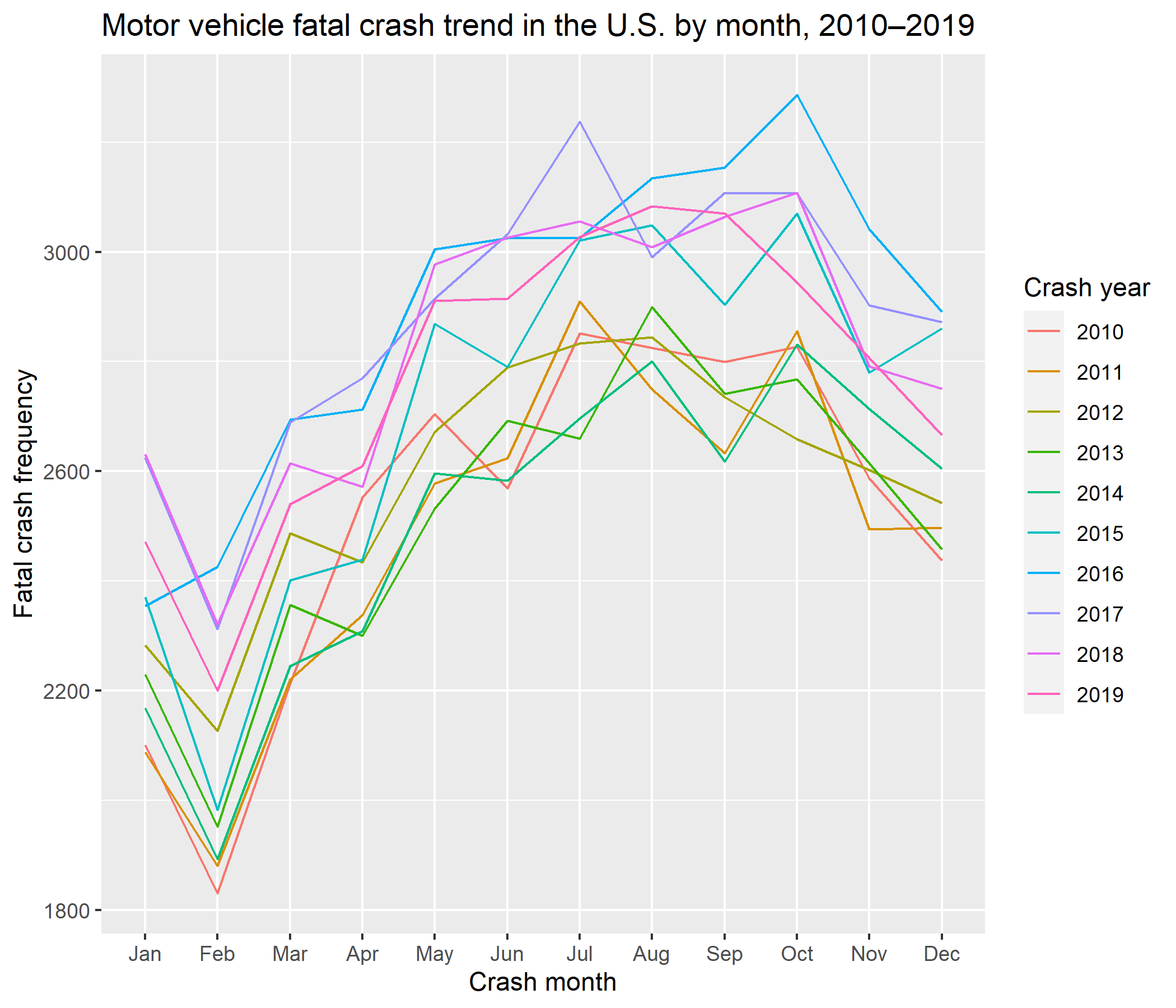
ggplot(fatal_crash_monthly_counts) + aes( x = crash_month, y = fatal_crash_freq ) + aes(group = crash_year) + geom_line() + scale_x_discrete(limits = month.abb) + aes(color = factor(crash_year)) + labs(x = "Crash month") + labs(y = "Fatal crash frequency") + labs(color = "Crash year") + labs( title = paste( "Motor vehicle fatal crash trend", "in the U.S. by month, 2010–2019" ) ) + labs(caption = "Data source: FARS")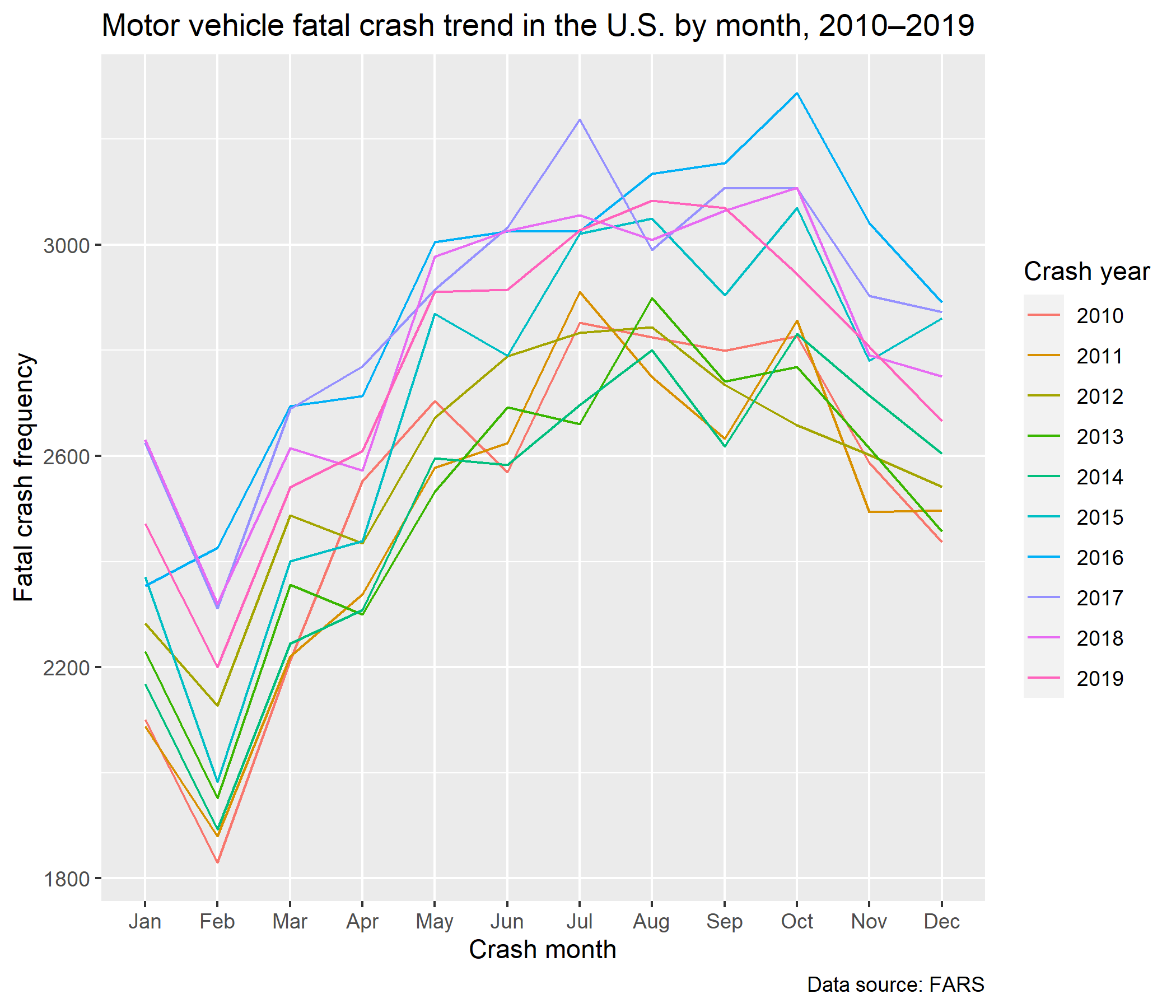
ggplot(fatal_crash_monthly_counts) + aes( x = crash_month, y = fatal_crash_freq ) + aes(group = crash_year) + geom_line() + scale_x_discrete(limits = month.abb) + aes(color = factor(crash_year)) + labs(x = "Crash month") + labs(y = "Fatal crash frequency") + labs(color = "Crash year") + labs( title = paste( "Motor vehicle fatal crash trend", "in the U.S. by month, 2010–2019" ) ) + labs(caption = "Data source: FARS") + gghighlight( max(fatal_crash_freq) > 3000 )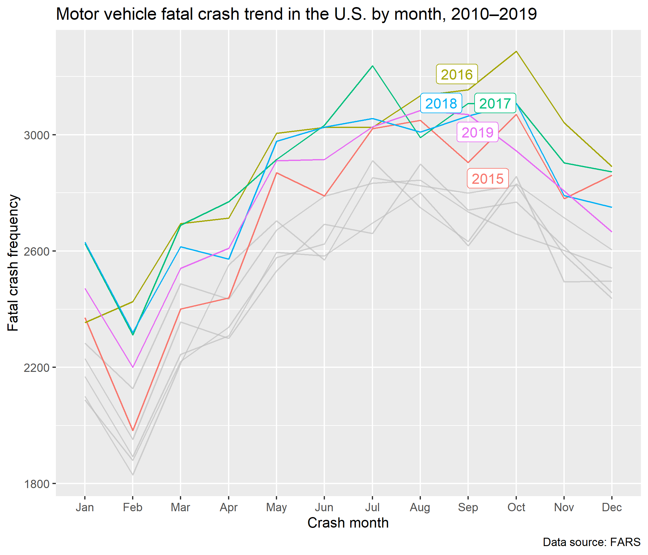
ggplot(fatal_crash_smry_by_state)
ggplot(fatal_crash_smry_by_state) + aes( x = death_rate_pop, y = death_rate_vmt )
ggplot(fatal_crash_smry_by_state) + aes( x = death_rate_pop, y = death_rate_vmt ) + geom_point()
ggplot(fatal_crash_smry_by_state) + aes( x = death_rate_pop, y = death_rate_vmt ) + geom_point() -> ggrepel_baseplotggrepel_baseplot
ggplot(fatal_crash_smry_by_state) + aes( x = death_rate_pop, y = death_rate_vmt ) + geom_point() -> ggrepel_baseplotggrepel_baseplot + geom_text(aes(label = state))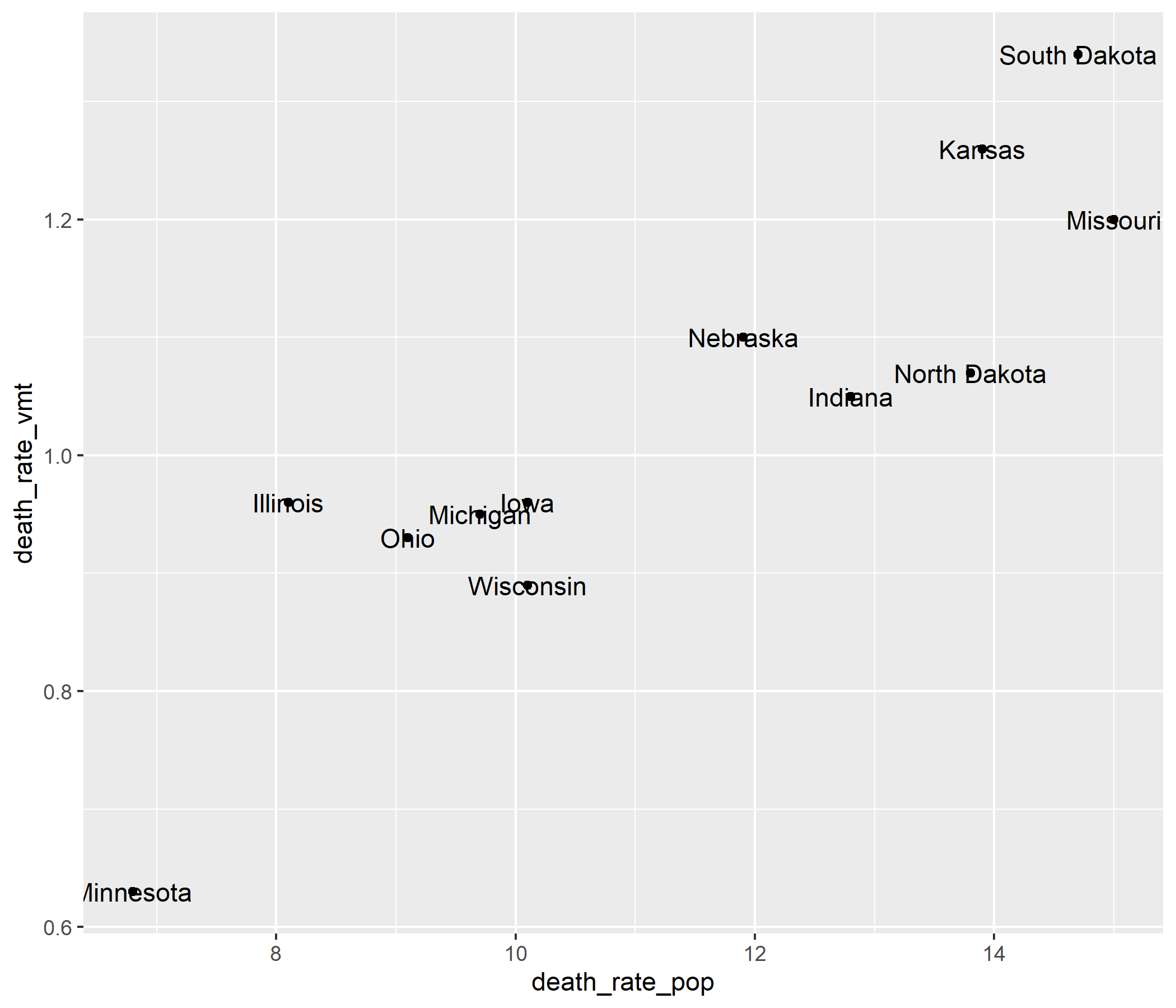
ggplot(fatal_crash_smry_by_state) + aes( x = death_rate_pop, y = death_rate_vmt ) + geom_point() -> ggrepel_baseplotggrepel_baseplot + geom_text(aes(label = state)) -> ggtext_uglyggrepel_baseplot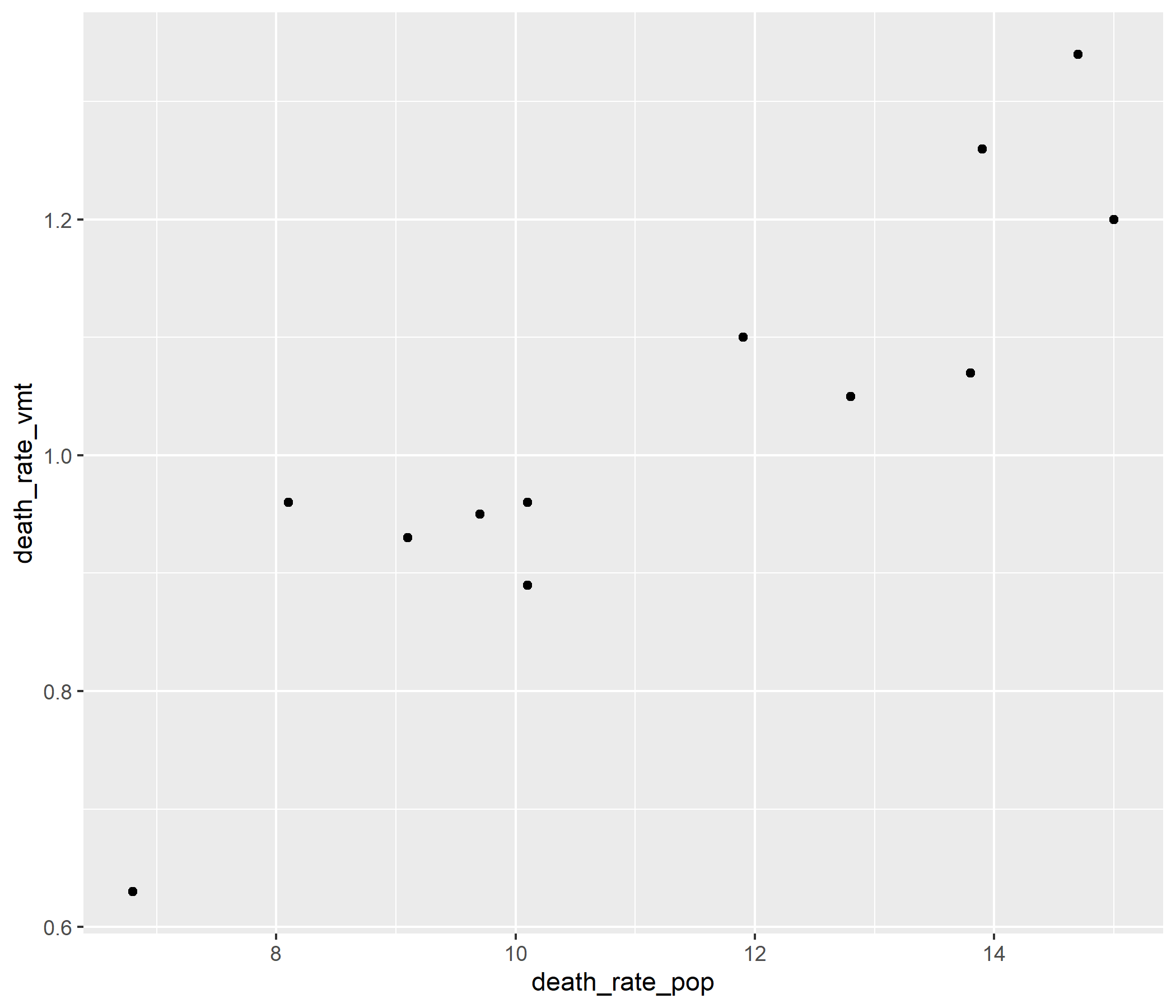
ggplot(fatal_crash_smry_by_state) + aes( x = death_rate_pop, y = death_rate_vmt ) + geom_point() -> ggrepel_baseplotggrepel_baseplot + geom_text(aes(label = state)) -> ggtext_uglyggrepel_baseplot + geom_text_repel( aes(label = state), seed = 123 )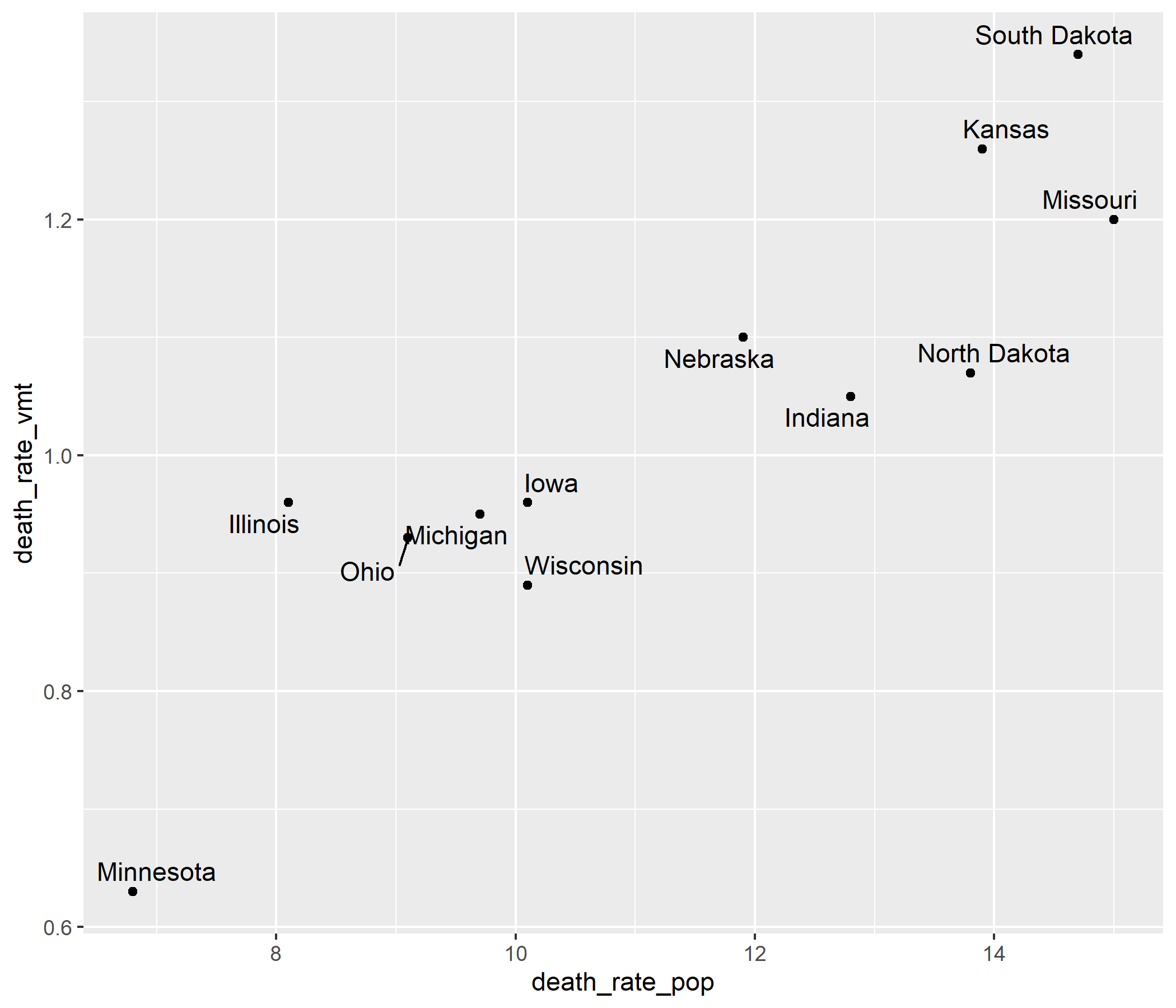
ggplot(fatal_crash_smry_by_state) + aes( x = death_rate_pop, y = death_rate_vmt ) + geom_point() -> ggrepel_baseplotggrepel_baseplot + geom_text(aes(label = state)) -> ggtext_uglyggrepel_baseplot + geom_text_repel( aes(label = state), seed = 123 ) -> ggtext_prettyggrepel_baseplot
ggplot(fatal_crash_smry_by_state) + aes( x = death_rate_pop, y = death_rate_vmt ) + geom_point() -> ggrepel_baseplotggrepel_baseplot + geom_text(aes(label = state)) -> ggtext_uglyggrepel_baseplot + geom_text_repel( aes(label = state), seed = 123 ) -> ggtext_prettyggrepel_baseplot + geom_label(aes(label = state))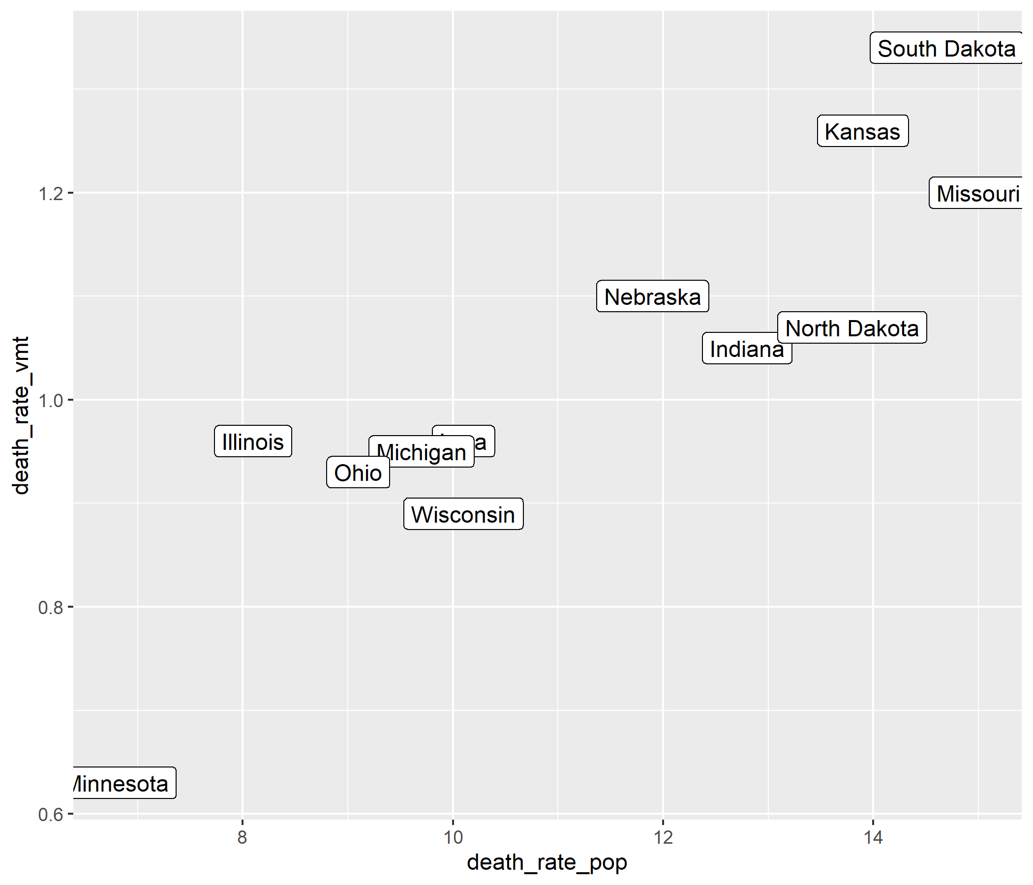
ggplot(fatal_crash_smry_by_state) + aes( x = death_rate_pop, y = death_rate_vmt ) + geom_point() -> ggrepel_baseplotggrepel_baseplot + geom_text(aes(label = state)) -> ggtext_uglyggrepel_baseplot + geom_text_repel( aes(label = state), seed = 123 ) -> ggtext_prettyggrepel_baseplot + geom_label(aes(label = state)) -> gglabel_uglyggrepel_baseplot
ggplot(fatal_crash_smry_by_state) + aes( x = death_rate_pop, y = death_rate_vmt ) + geom_point() -> ggrepel_baseplotggrepel_baseplot + geom_text(aes(label = state)) -> ggtext_uglyggrepel_baseplot + geom_text_repel( aes(label = state), seed = 123 ) -> ggtext_prettyggrepel_baseplot + geom_label(aes(label = state)) -> gglabel_uglyggrepel_baseplot + geom_label_repel( aes(label = state), seed = 123 )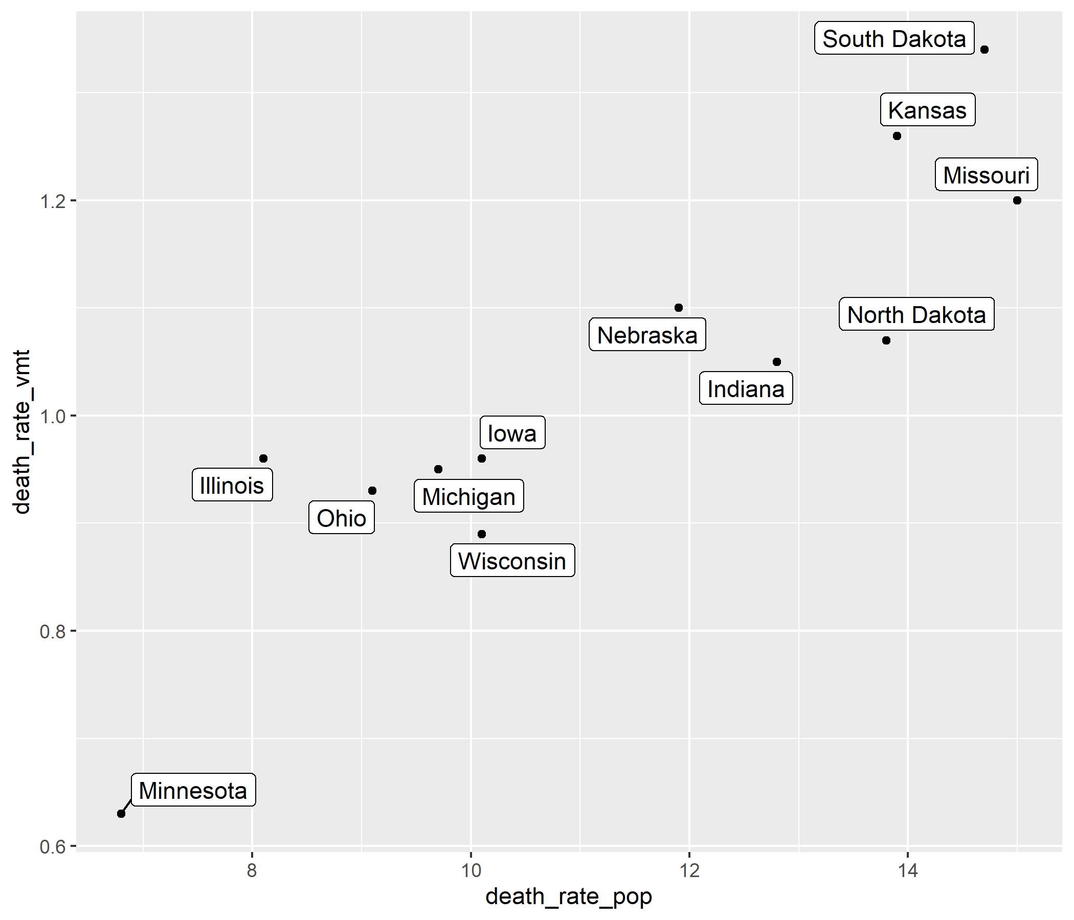
ggrepel_baseplot + geom_label_repel( aes(label = state), seed = 123, ) + geom_smooth( method = "lm", se = FALSE ) + labs( x = "Deaths per 100k population" ) + labs( y = "Deaths per 100 million VMT" ) + labs( title = paste( "Relationship between motor", "vehicle crash death rates", "for midwest, 2018" ) ) + labs(caption = "Data source: IIHS")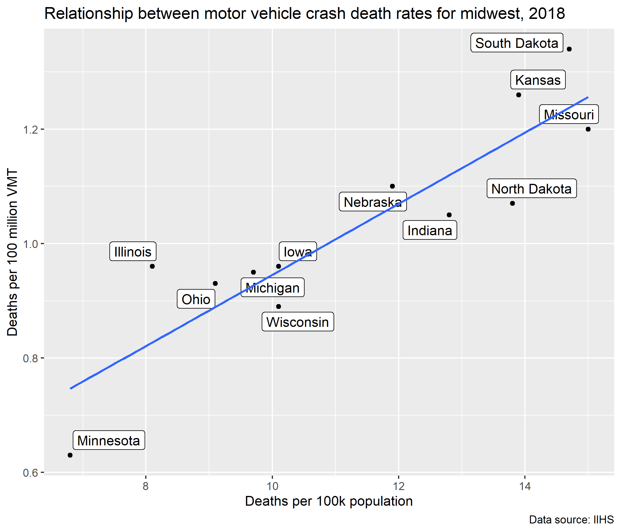
ggrepel_baseplot + geom_label_repel( aes(label = state), seed = 123, nudge_x = 0.2, ) + geom_smooth( method = "lm", se = FALSE ) + labs( x = "Deaths per 100k population" ) + labs( y = "Deaths per 100 million VMT" ) + labs( title = paste( "Relationship between motor", "vehicle crash death rates", "for midwest, 2018" ) ) + labs(caption = "Data source: IIHS")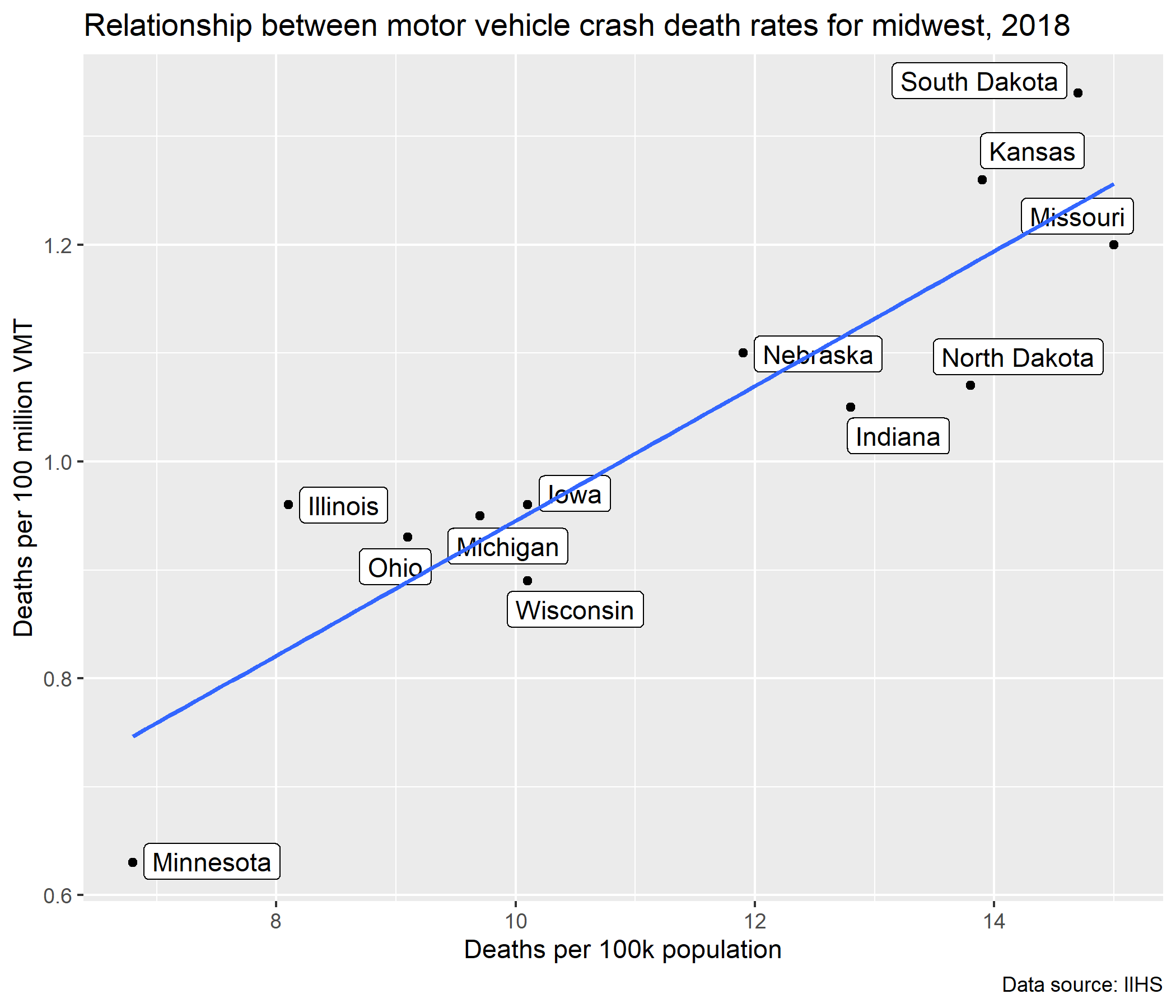
ggrepel_baseplot + geom_label_repel( aes(label = state), seed = 123, nudge_x = 0.2, box.padding = 1, ) + geom_smooth( method = "lm", se = FALSE ) + labs( x = "Deaths per 100k population" ) + labs( y = "Deaths per 100 million VMT" ) + labs( title = paste( "Relationship between motor", "vehicle crash death rates", "for midwest, 2018" ) ) + labs(caption = "Data source: IIHS")
ggrepel_baseplot + geom_label_repel( aes(label = state), seed = 123, nudge_x = 0.2, box.padding = 1, segment.curvature = -0.2, ) + geom_smooth( method = "lm", se = FALSE ) + labs( x = "Deaths per 100k population" ) + labs( y = "Deaths per 100 million VMT" ) + labs( title = paste( "Relationship between motor", "vehicle crash death rates", "for midwest, 2018" ) ) + labs(caption = "Data source: IIHS")
ggrepel_baseplot + geom_label_repel( aes(label = state), seed = 123, nudge_x = 0.2, box.padding = 1, segment.curvature = -0.2, segment.ncp = 5, ) + geom_smooth( method = "lm", se = FALSE ) + labs( x = "Deaths per 100k population" ) + labs( y = "Deaths per 100 million VMT" ) + labs( title = paste( "Relationship between motor", "vehicle crash death rates", "for midwest, 2018" ) ) + labs(caption = "Data source: IIHS")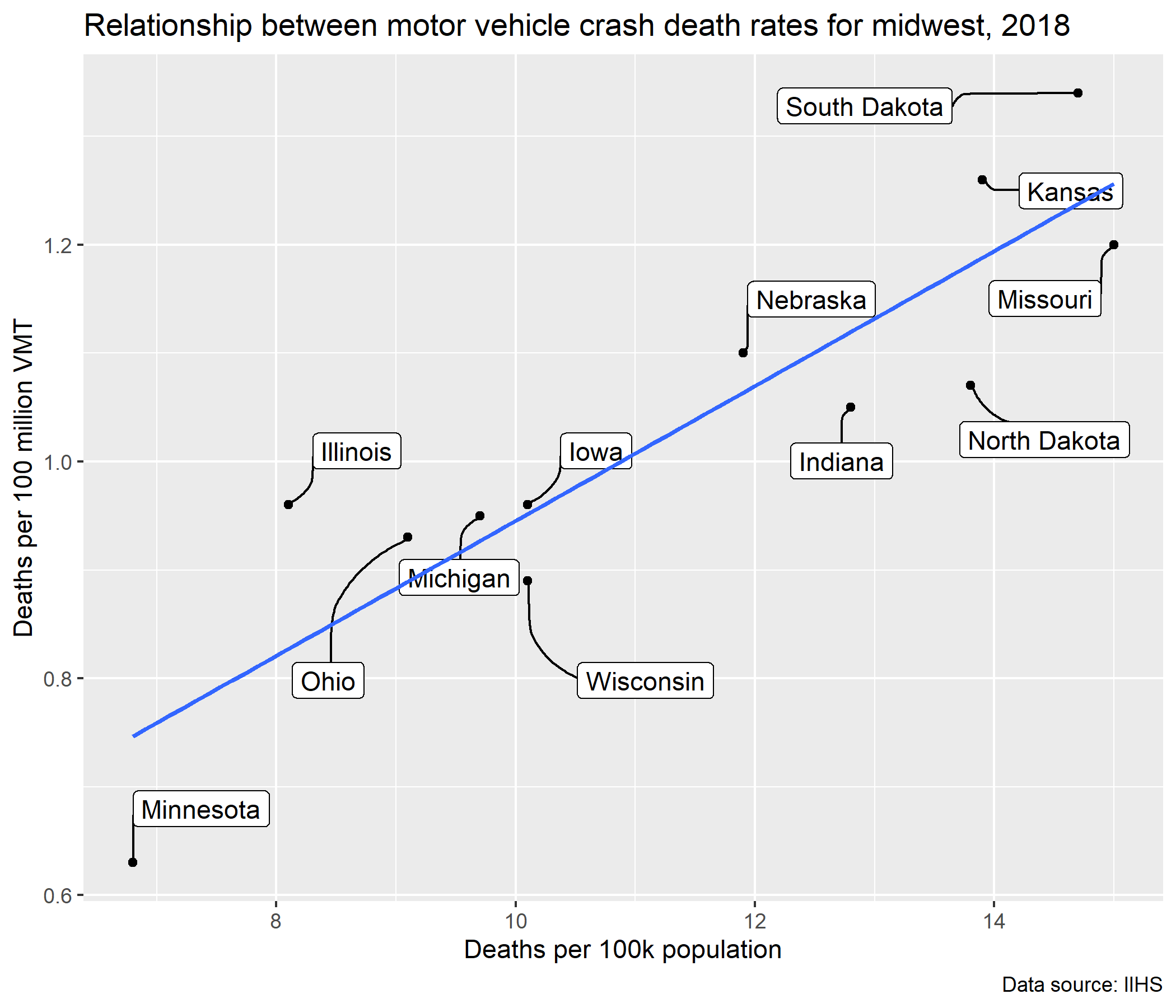
ggrepel_baseplot + geom_label_repel( aes(label = state), seed = 123, nudge_x = 0.2, box.padding = 1, segment.curvature = -0.2, segment.ncp = 5, segment.angle = 30 ) + geom_smooth( method = "lm", se = FALSE ) + labs( x = "Deaths per 100k population" ) + labs( y = "Deaths per 100 million VMT" ) + labs( title = paste( "Relationship between motor", "vehicle crash death rates", "for midwest, 2018" ) ) + labs(caption = "Data source: IIHS")
lol_chart <- ggdotchart( data = fatal_crash_smry_by_state, x = "state", y = "death_rate_vmt",)lol_chart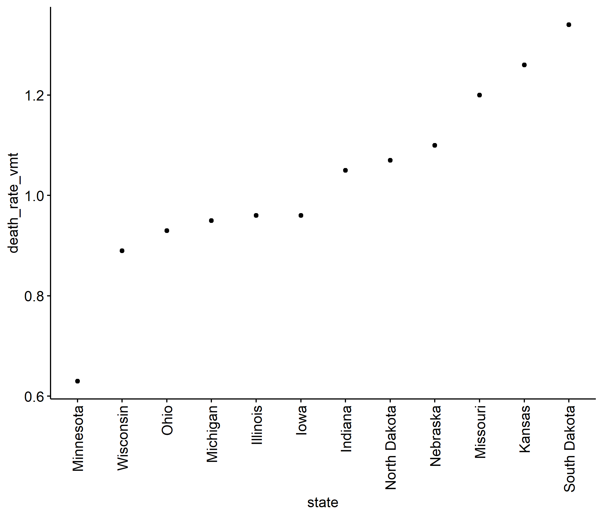
lol_chart <- ggdotchart( data = fatal_crash_smry_by_state, x = "state", y = "death_rate_vmt", sorting = "descending",)lol_chart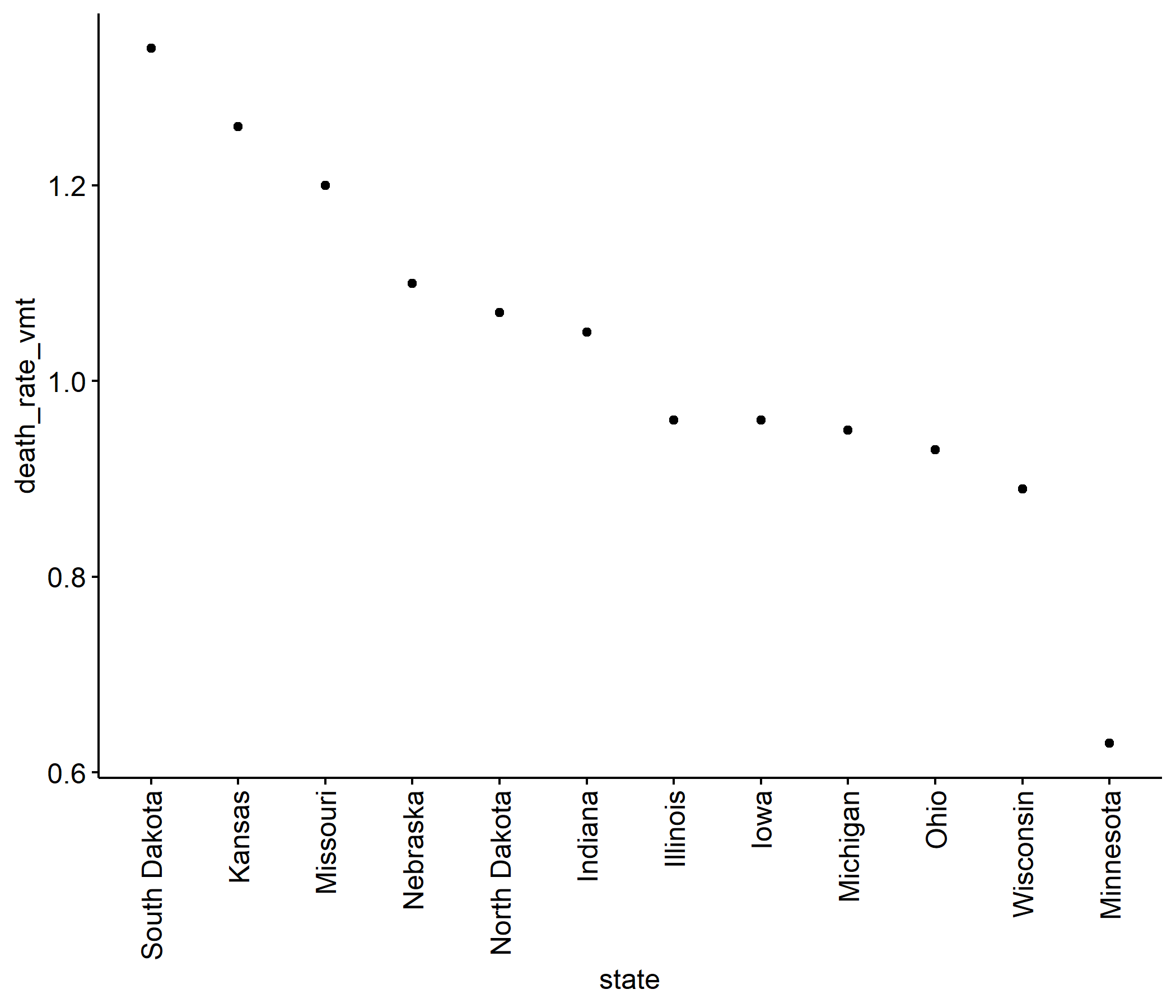
lol_chart <- ggdotchart( data = fatal_crash_smry_by_state, x = "state", y = "death_rate_vmt", sorting = "descending", add = "segment",)lol_chart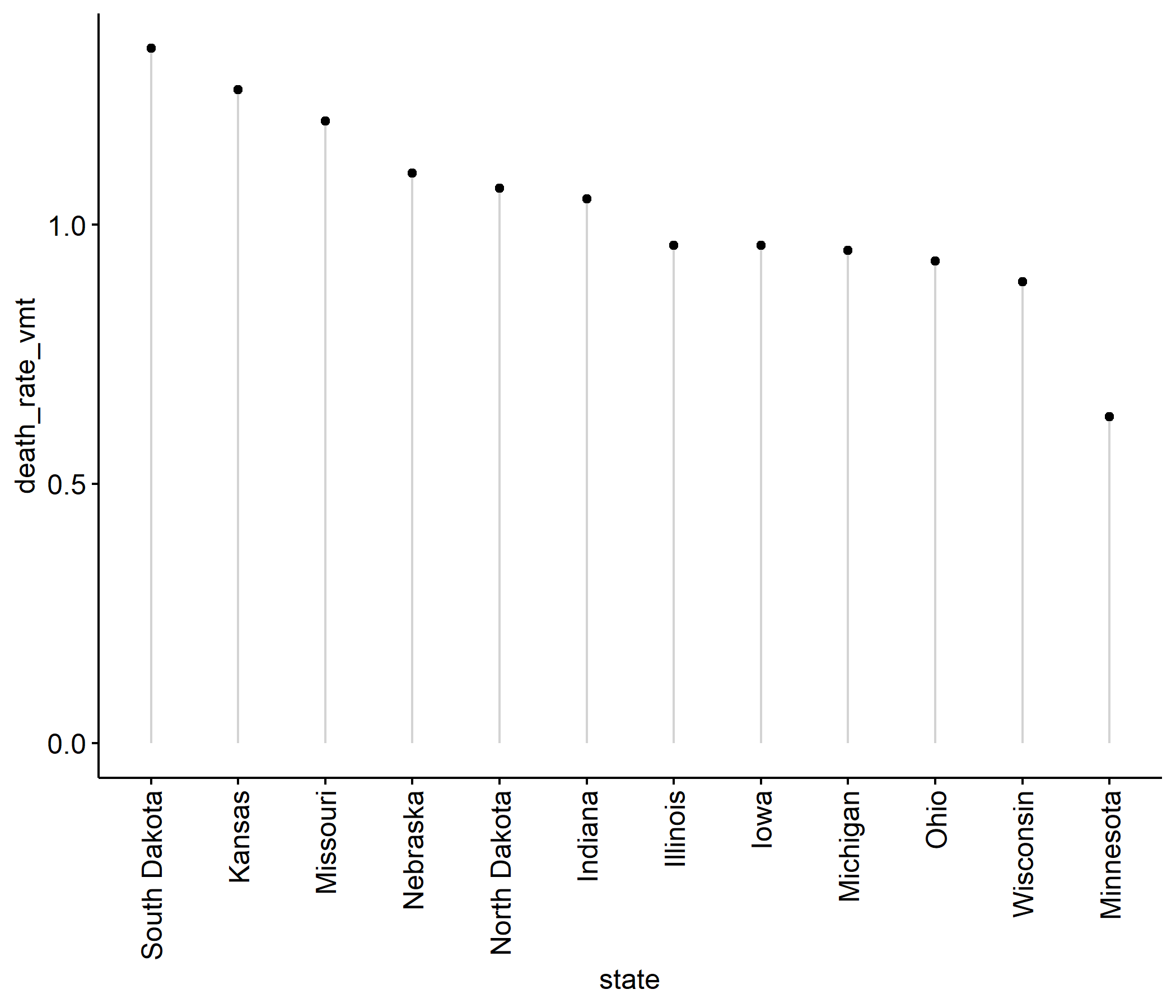
lol_chart <- ggdotchart( data = fatal_crash_smry_by_state, x = "state", y = "death_rate_vmt", sorting = "descending", add = "segment", add.params = list(size = 1),)lol_chart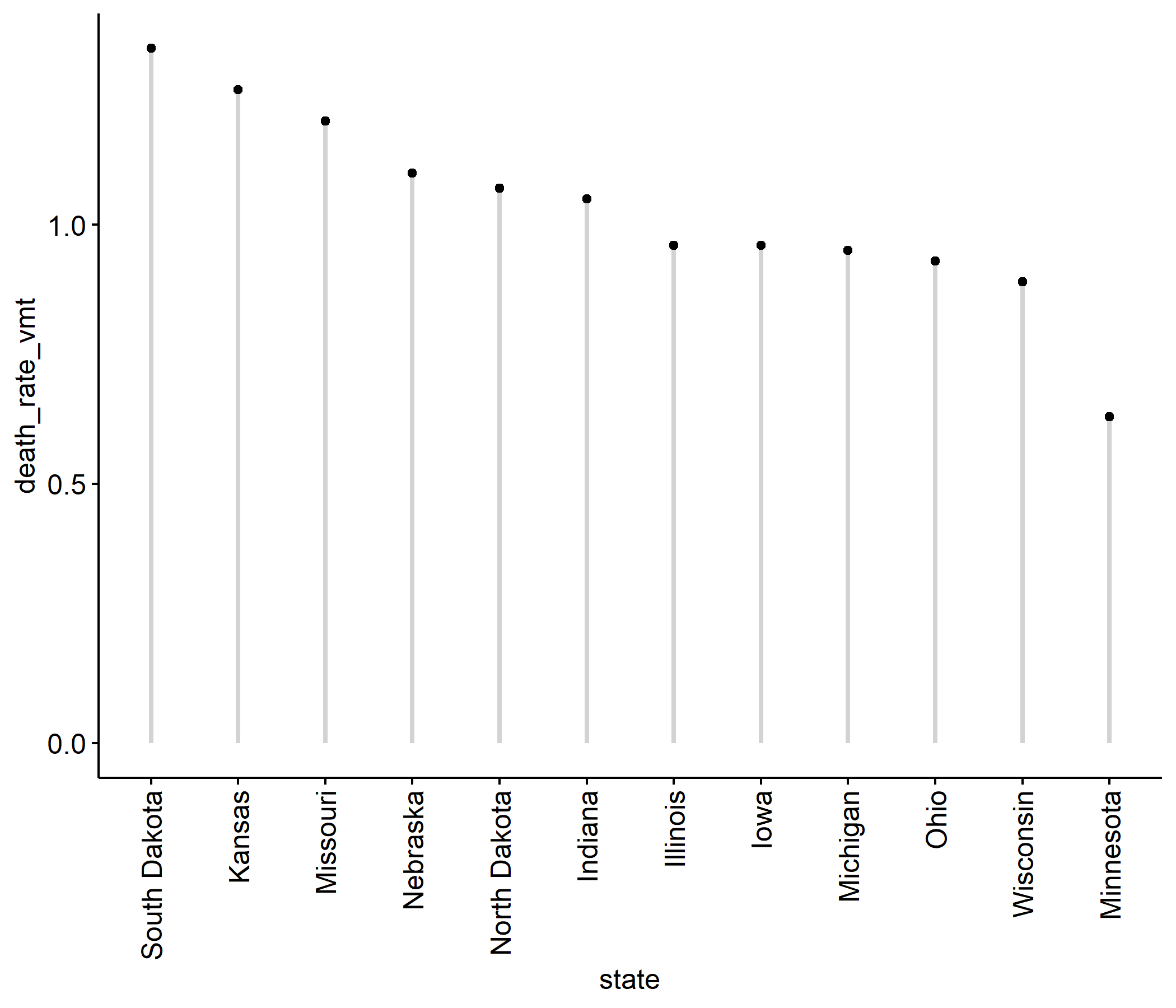
lol_chart <- ggdotchart( data = fatal_crash_smry_by_state, x = "state", y = "death_rate_vmt", sorting = "descending", add = "segment", add.params = list(size = 1), dot.size = 9,)lol_chart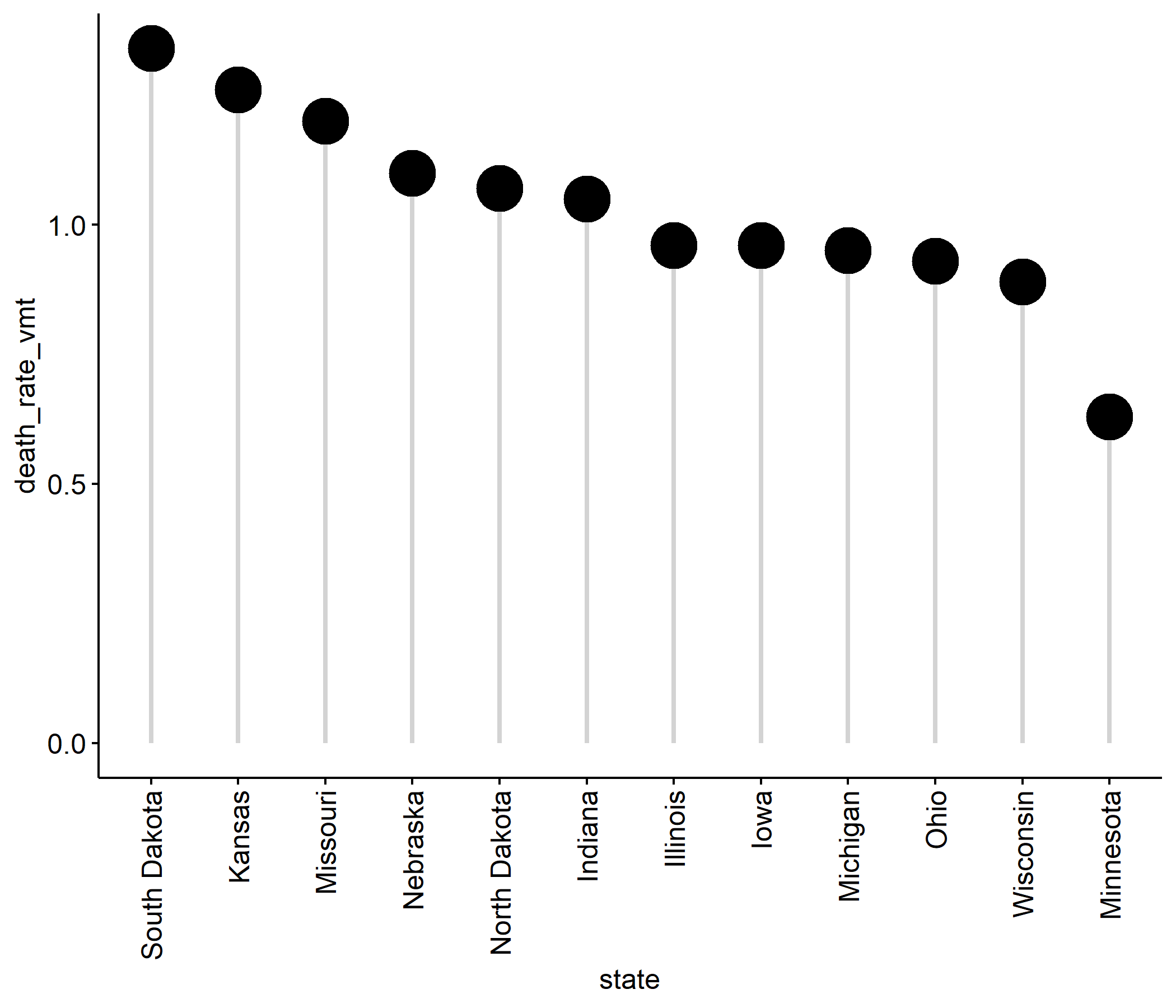
lol_chart <- ggdotchart( data = fatal_crash_smry_by_state, x = "state", y = "death_rate_vmt", sorting = "descending", add = "segment", add.params = list(size = 1), dot.size = 9, rotate = TRUE,)lol_chart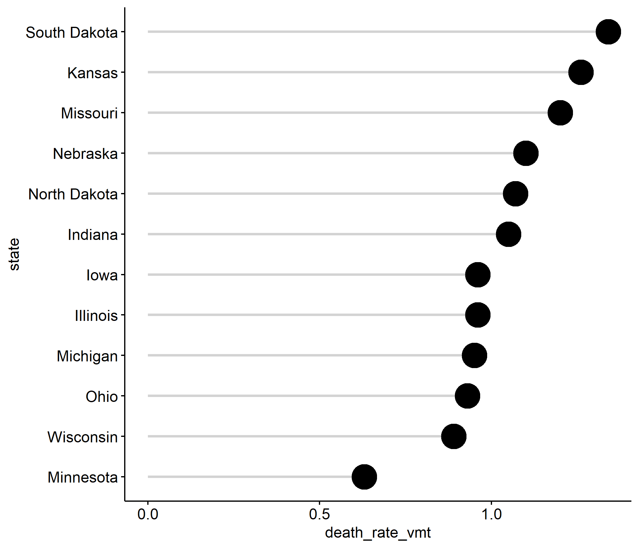
lol_chart <- ggdotchart( data = fatal_crash_smry_by_state, x = "state", y = "death_rate_vmt", sorting = "descending", add = "segment", add.params = list(size = 1), dot.size = 9, rotate = TRUE, color = "death_rate_vmt_above_mean",)lol_chart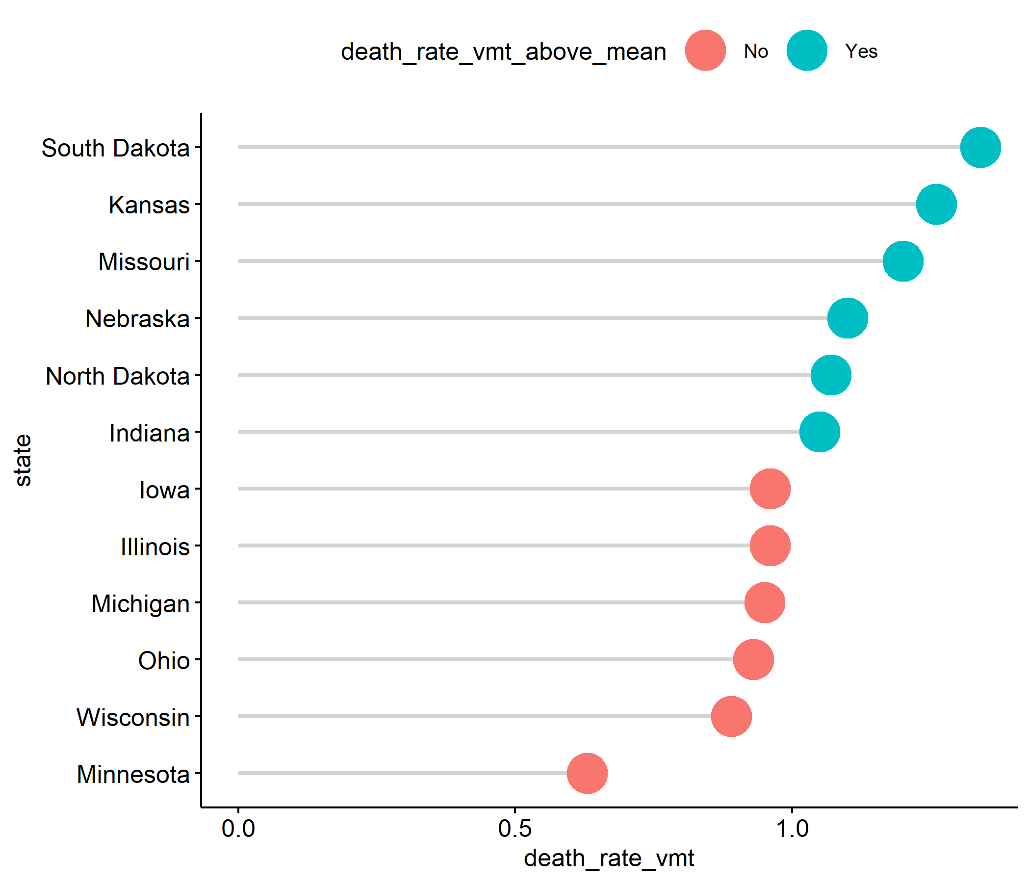
lol_chart <- ggdotchart( data = fatal_crash_smry_by_state, x = "state", y = "death_rate_vmt", sorting = "descending", add = "segment", add.params = list(size = 1), dot.size = 9, rotate = TRUE, color = "death_rate_vmt_above_mean", label = "death_rate_vmt", font.label = list( color = "white", size = 9, vjust = 0.5 ),)lol_chart
lol_chart <- ggdotchart( data = fatal_crash_smry_by_state, x = "state", y = "death_rate_vmt", sorting = "descending", add = "segment", add.params = list(size = 1), dot.size = 9, rotate = TRUE, color = "death_rate_vmt_above_mean", label = "death_rate_vmt", font.label = list( color = "white", size = 9, vjust = 0.5 ), legend.title = "Value above mean", title = paste( "Motor vehicle crash death rate", "per midwestern state, 2018" ), xlab = "Midwestern state", ylab = "Deaths per 100 million VMT", caption = "Data source: IIHS")lol_chart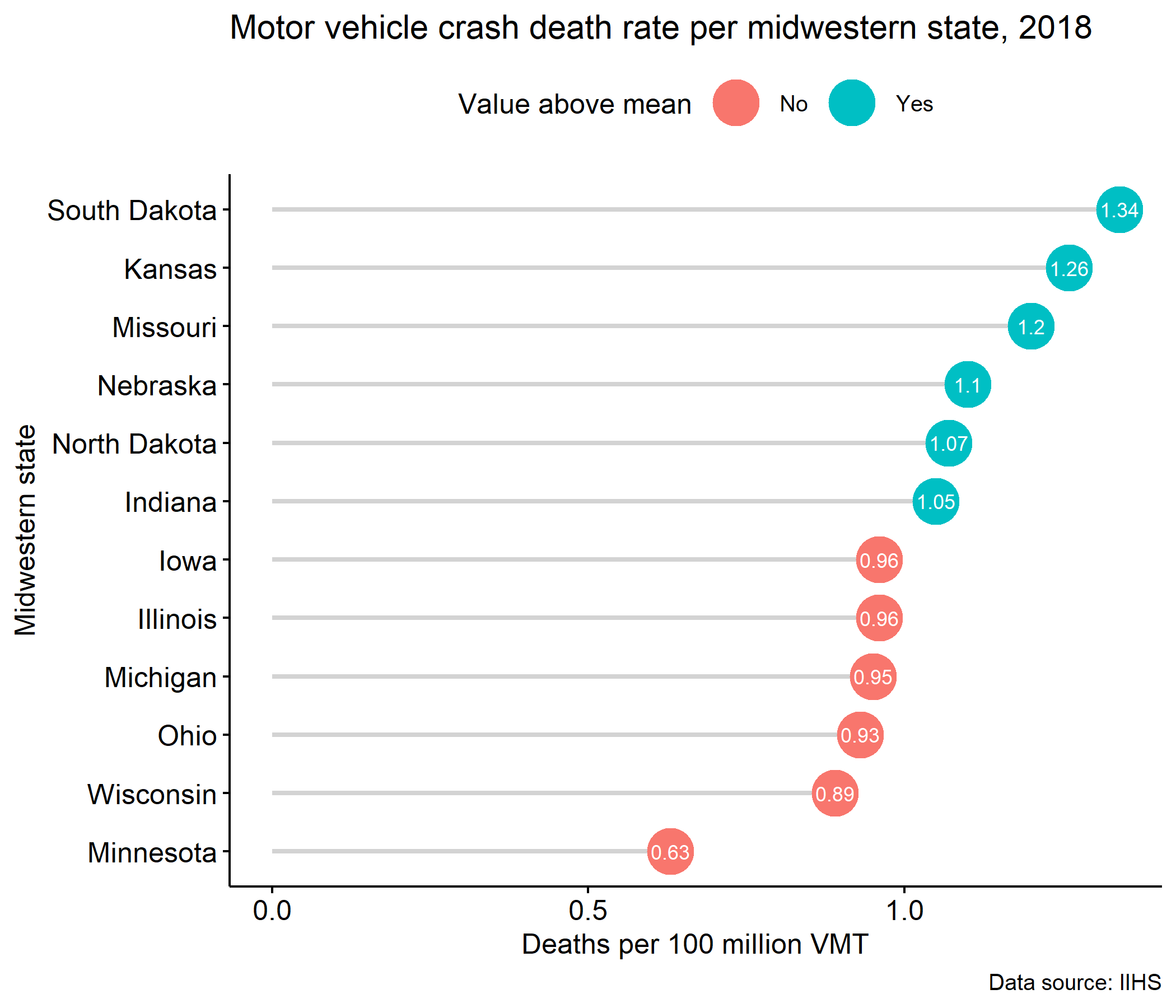
dev_chart <- ggdotchart( data = fatal_crash_smry_by_state, x = "state", y = "death_rate_vmt_z",) + geom_hline( yintercept = 0, )dev_chart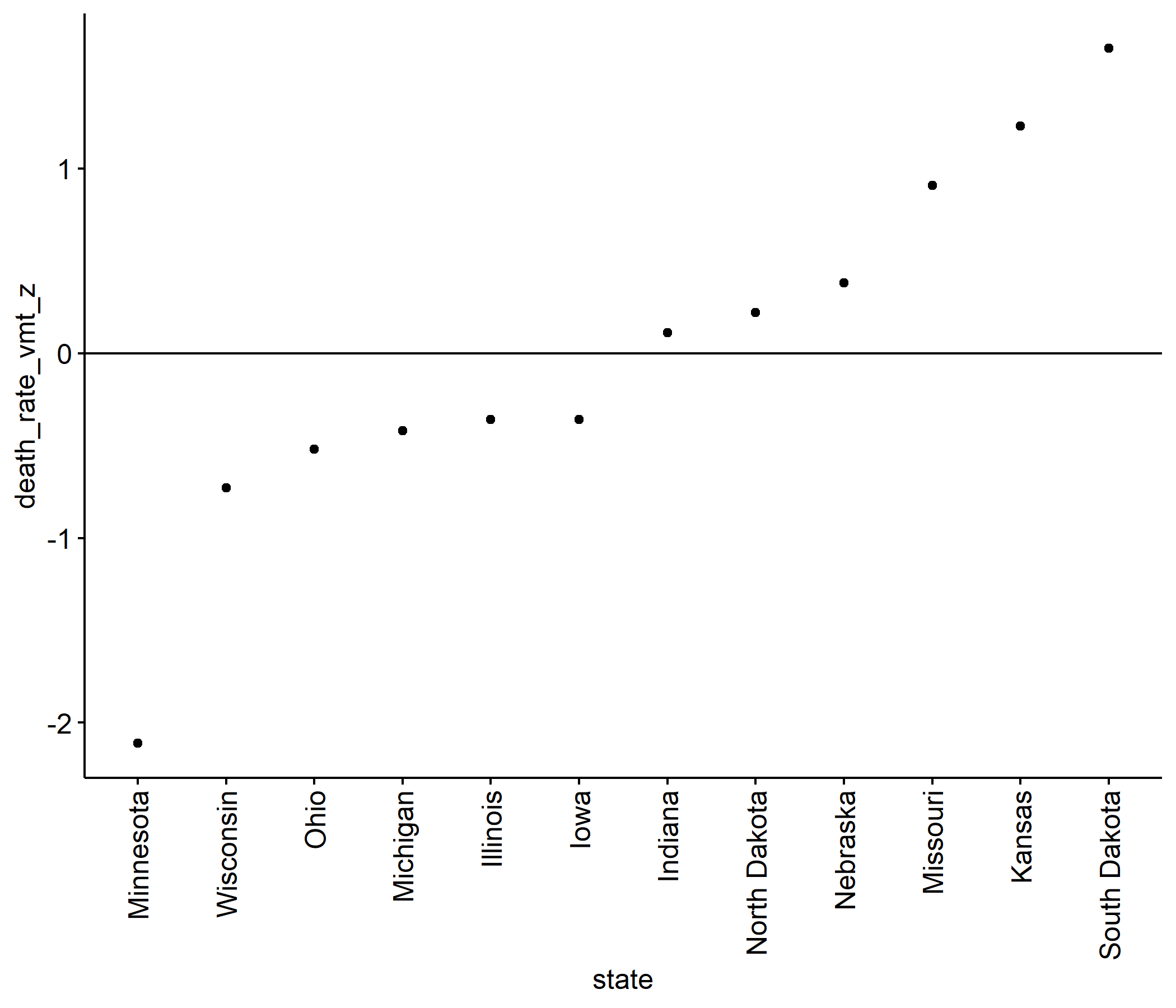
dev_chart <- ggdotchart( data = fatal_crash_smry_by_state, x = "state", y = "death_rate_vmt_z", sorting = "descending",) + geom_hline( yintercept = 0, )dev_chart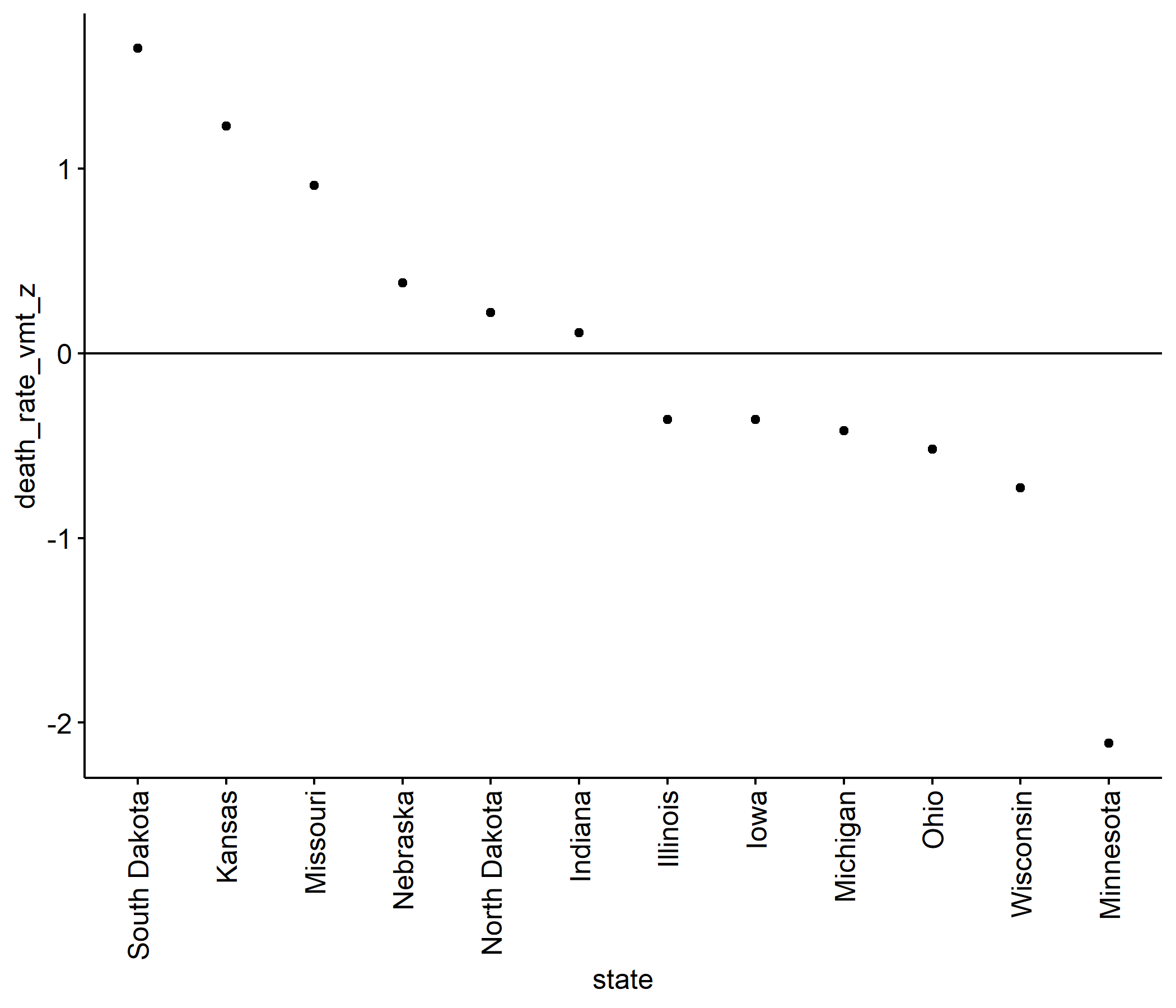
dev_chart <- ggdotchart( data = fatal_crash_smry_by_state, x = "state", y = "death_rate_vmt_z", sorting = "descending", add = "segment",) + geom_hline( yintercept = 0, )dev_chart
dev_chart <- ggdotchart( data = fatal_crash_smry_by_state, x = "state", y = "death_rate_vmt_z", sorting = "descending", add = "segment", add.params = list(size = 2),) + geom_hline( yintercept = 0, )dev_chart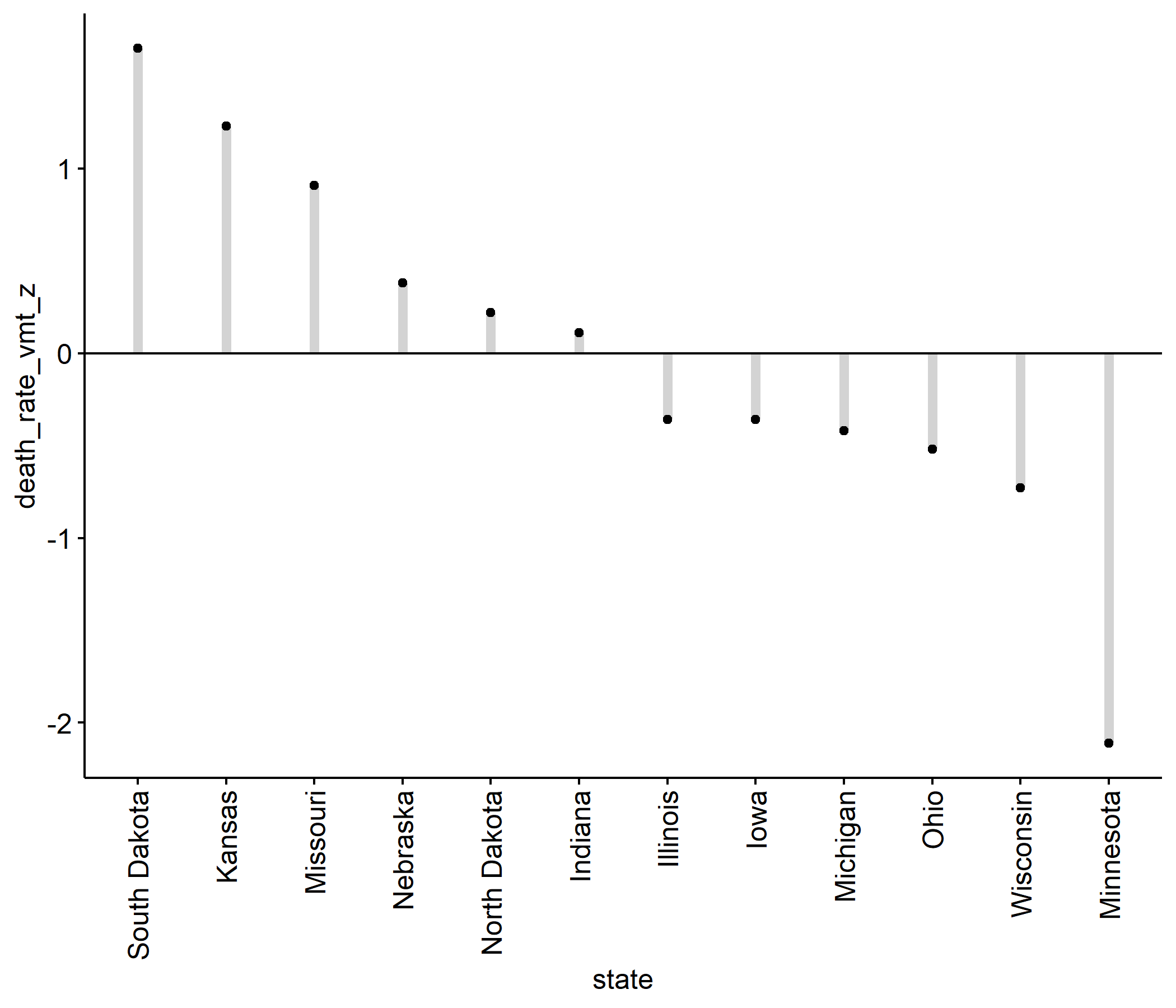
dev_chart <- ggdotchart( data = fatal_crash_smry_by_state, x = "state", y = "death_rate_vmt_z", sorting = "descending", add = "segment", add.params = list(size = 2), dot.size = 9, rotate = TRUE,) + geom_hline( yintercept = 0, )dev_chart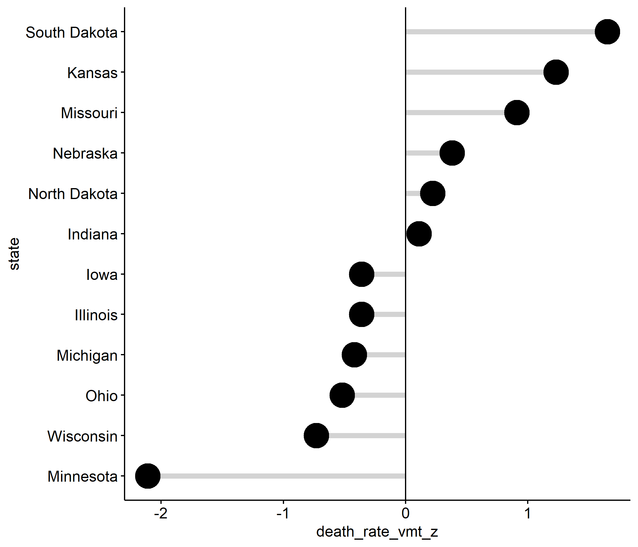
dev_chart <- ggdotchart( data = fatal_crash_smry_by_state, x = "state", y = "death_rate_vmt_z", sorting = "descending", add = "segment", add.params = list(size = 2), dot.size = 9, rotate = TRUE, color = "death_rate_vmt_above_mean",) + geom_hline( yintercept = 0, )dev_chart
dev_chart <- ggdotchart( data = fatal_crash_smry_by_state, x = "state", y = "death_rate_vmt_z", sorting = "descending", add = "segment", add.params = list(size = 2), dot.size = 9, rotate = TRUE, color = "death_rate_vmt_above_mean", label = "death_rate_vmt_z",) + geom_hline( yintercept = 0, )dev_chart
dev_chart <- ggdotchart( data = fatal_crash_smry_by_state, x = "state", y = "death_rate_vmt_z", sorting = "descending", add = "segment", add.params = list(size = 2), dot.size = 9, rotate = TRUE, color = "death_rate_vmt_above_mean", label = "death_rate_vmt_z", font.label = list( color = "white", size = 9, vjust = 0.5 ),) + geom_hline( yintercept = 0, )dev_chart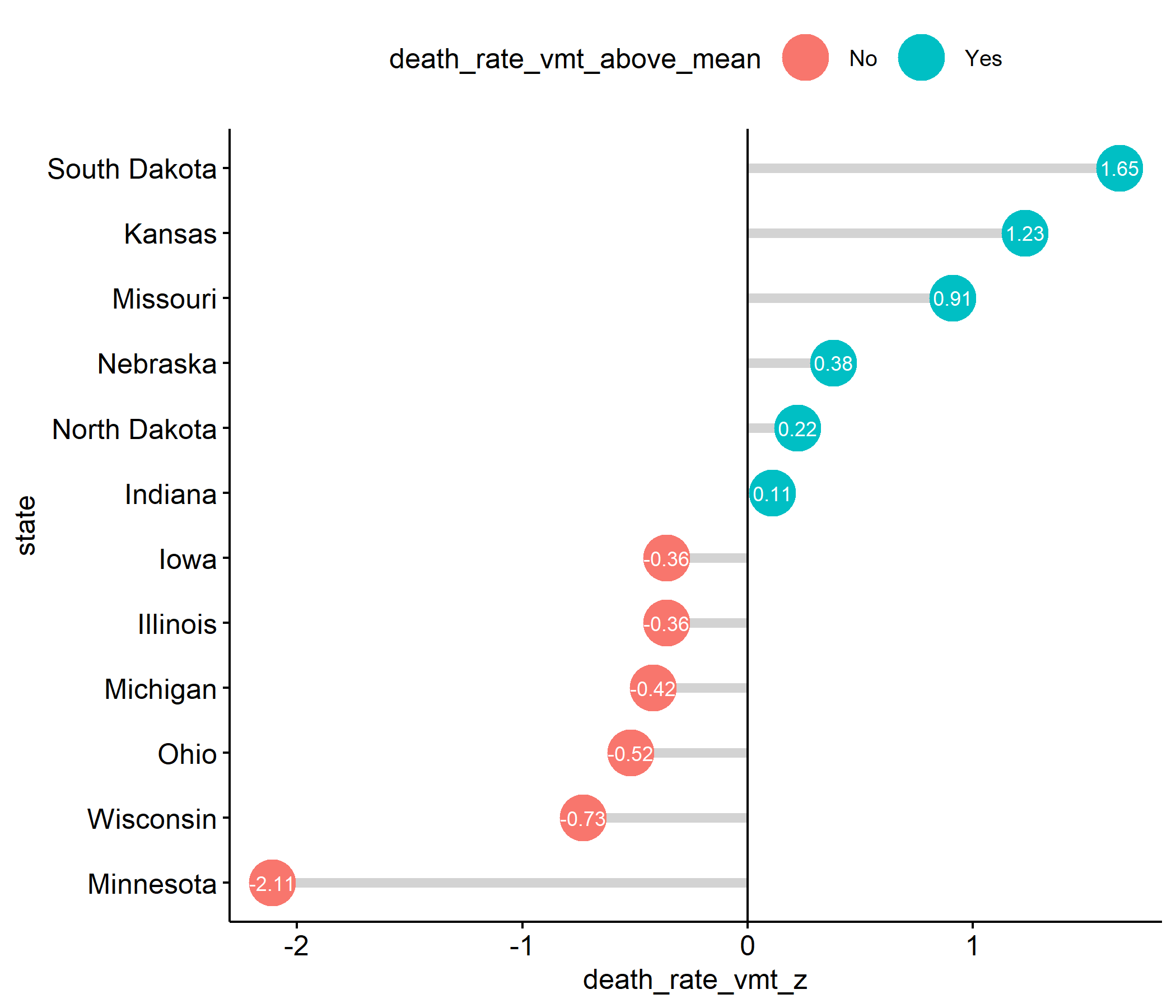
dev_chart <- ggdotchart( data = fatal_crash_smry_by_state, x = "state", y = "death_rate_vmt_z", sorting = "descending", add = "segment", add.params = list(size = 2), dot.size = 9, rotate = TRUE, color = "death_rate_vmt_above_mean", label = "death_rate_vmt_z", font.label = list( color = "white", size = 9, vjust = 0.5 ), legend.title = "Value above mean", title = paste( "Motor vehicle crash death", "rate per midwestern state, 2018" ), xlab = "Midwestern state", ylab = paste( "Deaths per 100 million VMT", "(normalized)" )) + geom_hline( yintercept = 0, linetype = 2, color = "lightgrey" )dev_chart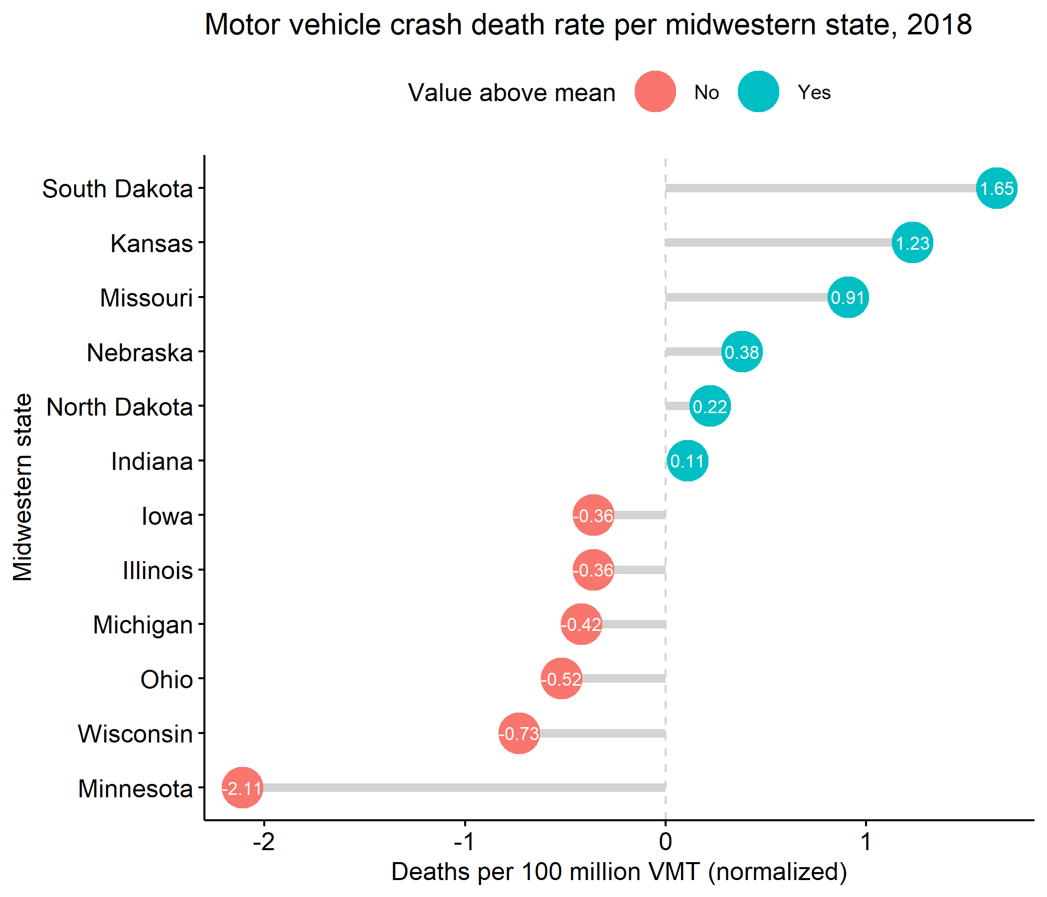
fatal_crash_monthly_counts %>% filter( crash_year %in% c(2015:2019) ) %>% ggviolin( x = "crash_year", y = "fatal_crash_freq", )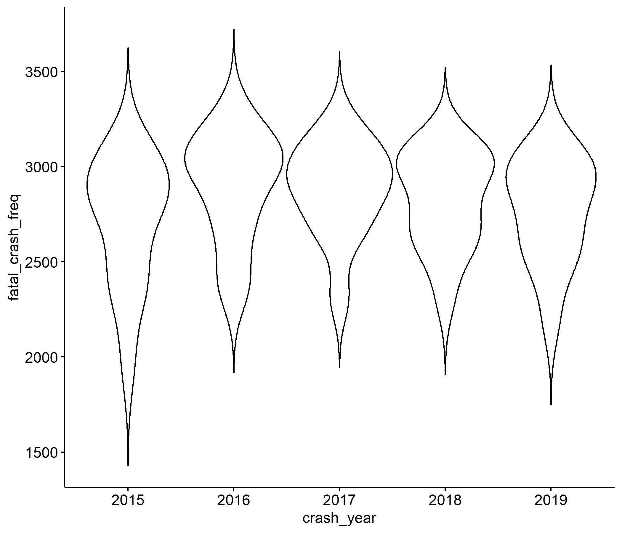
fatal_crash_monthly_counts %>% filter( crash_year %in% c(2015:2019) ) %>% ggviolin( x = "crash_year", y = "fatal_crash_freq", fill = "crash_year", )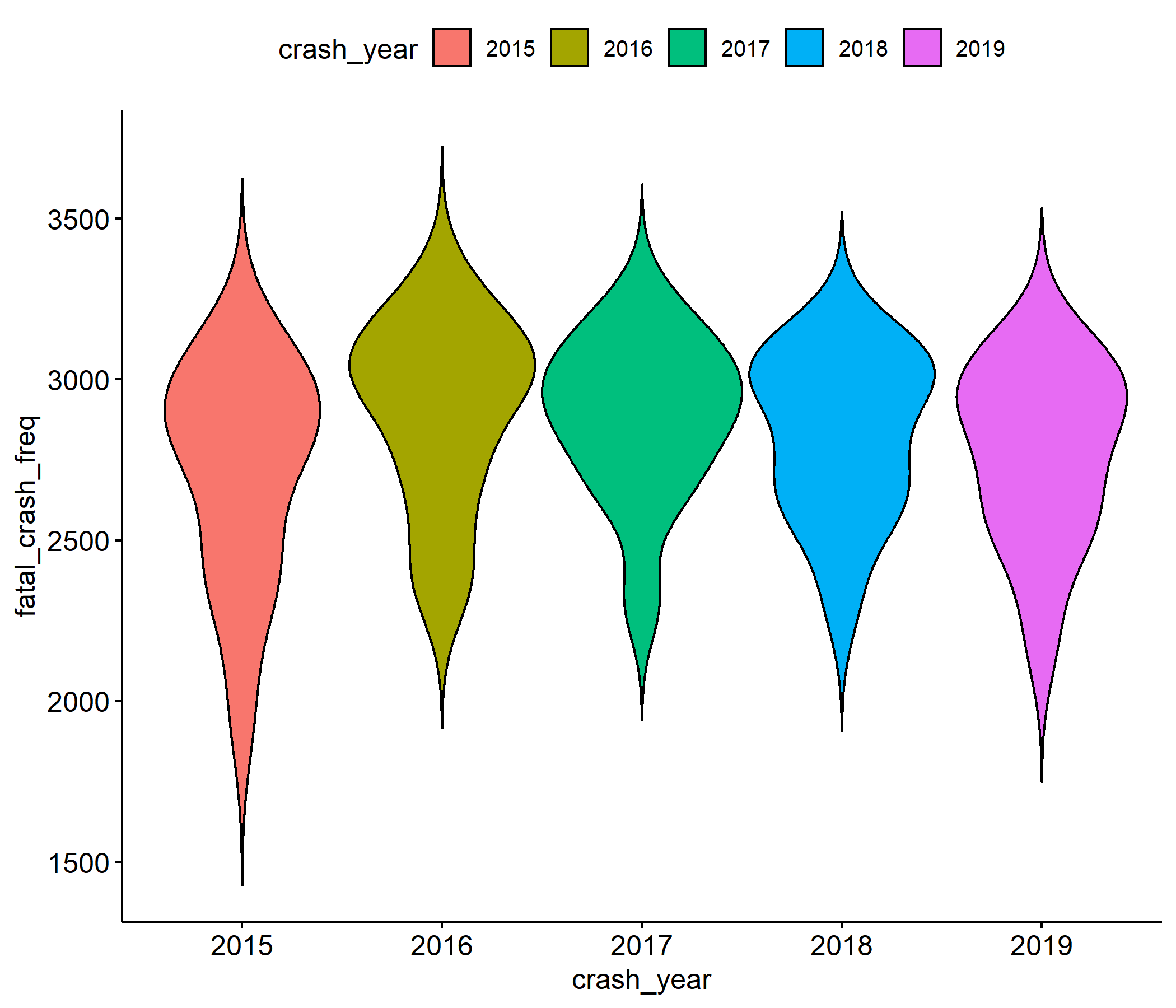
fatal_crash_monthly_counts %>% filter( crash_year %in% c(2015:2019) ) %>% ggviolin( x = "crash_year", y = "fatal_crash_freq", fill = "crash_year", palette = plasma( 5, begin = 0.4, end = 0.8 ), )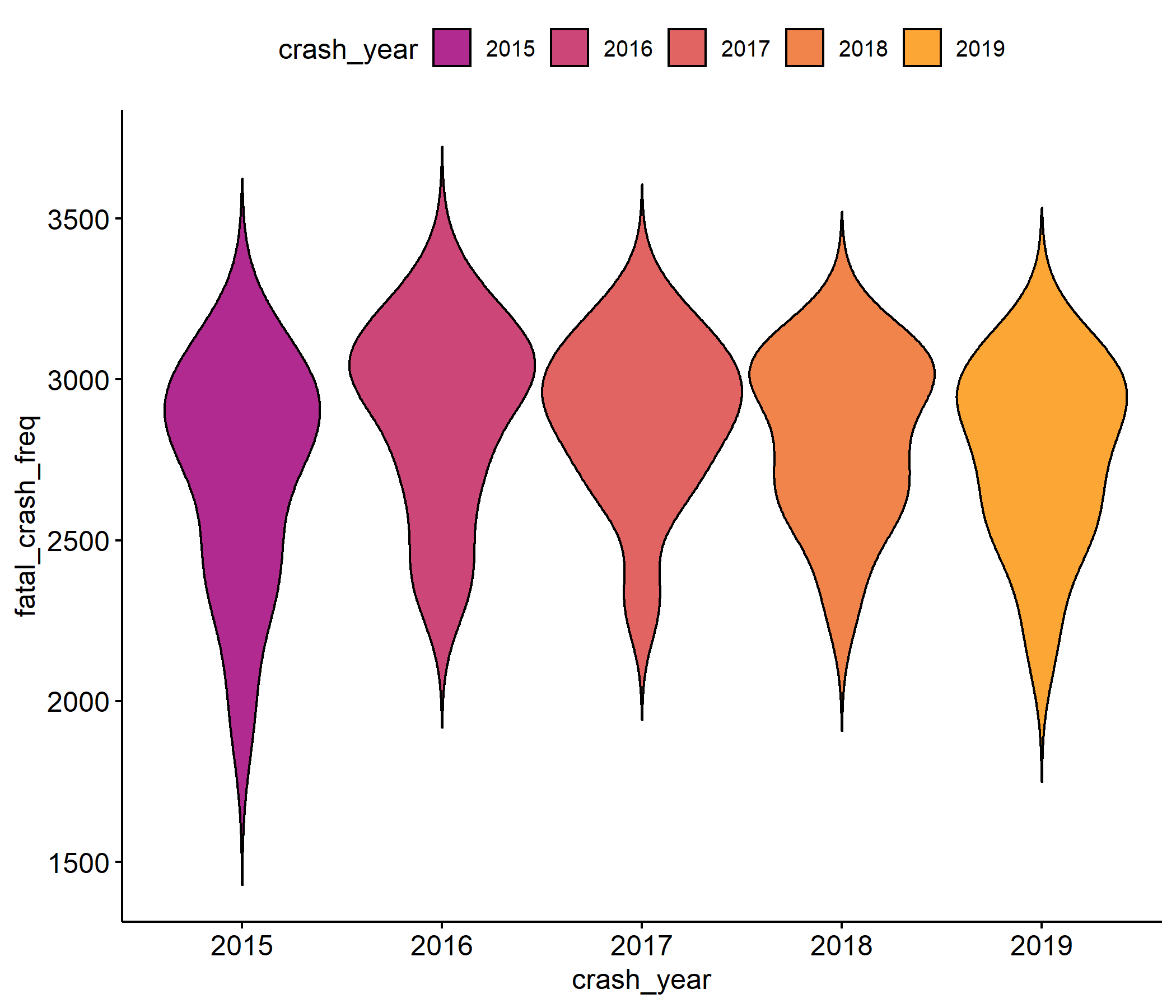
fatal_crash_monthly_counts %>% filter( crash_year %in% c(2015:2019) ) %>% ggviolin( x = "crash_year", y = "fatal_crash_freq", fill = "crash_year", palette = plasma( 5, begin = 0.4, end = 0.8 ), add = "boxplot", )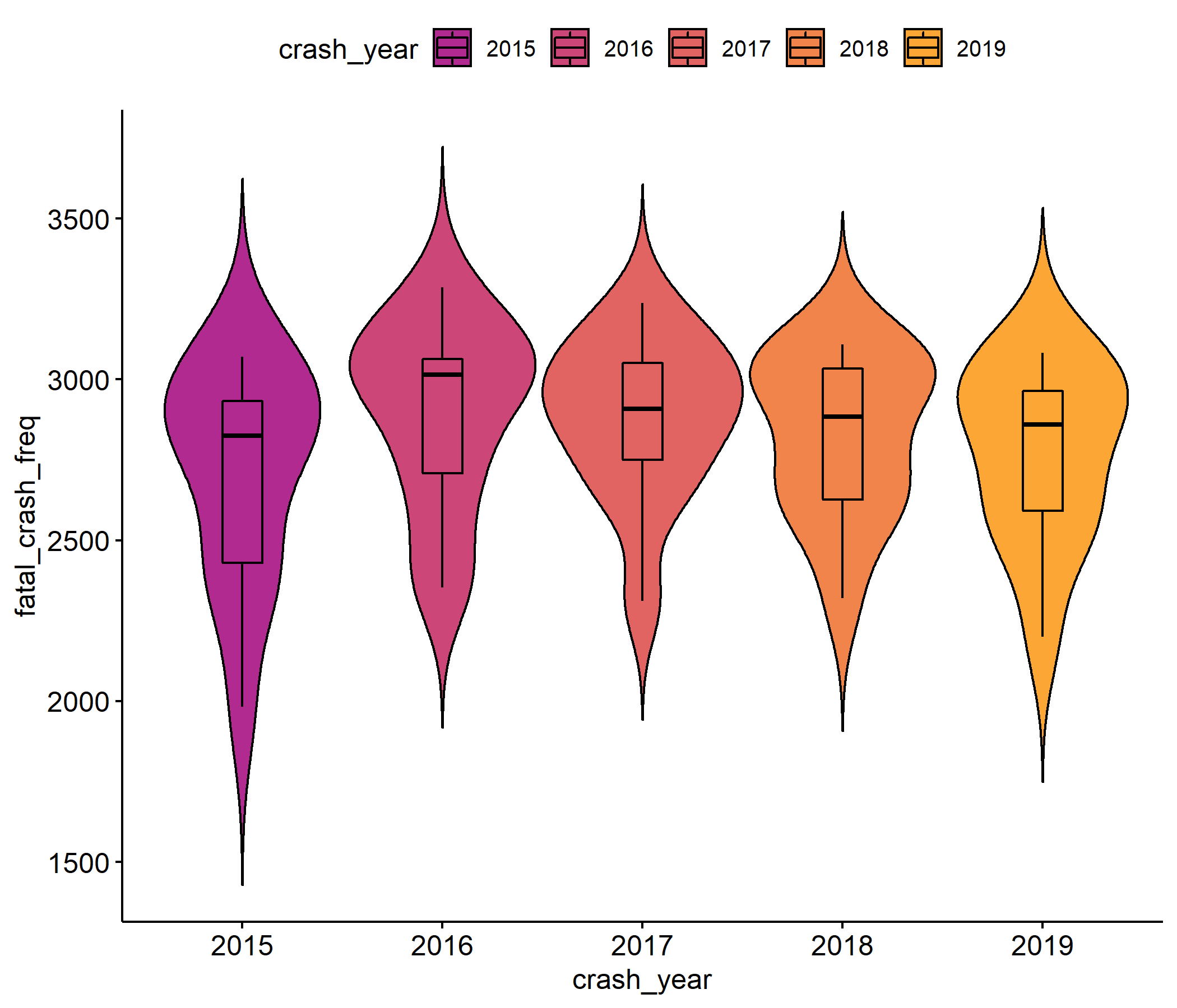
fatal_crash_monthly_counts %>% filter( crash_year %in% c(2015:2019) ) %>% ggviolin( x = "crash_year", y = "fatal_crash_freq", fill = "crash_year", palette = plasma( 5, begin = 0.4, end = 0.8 ), add = "boxplot", add.params = list(fill = "white"), )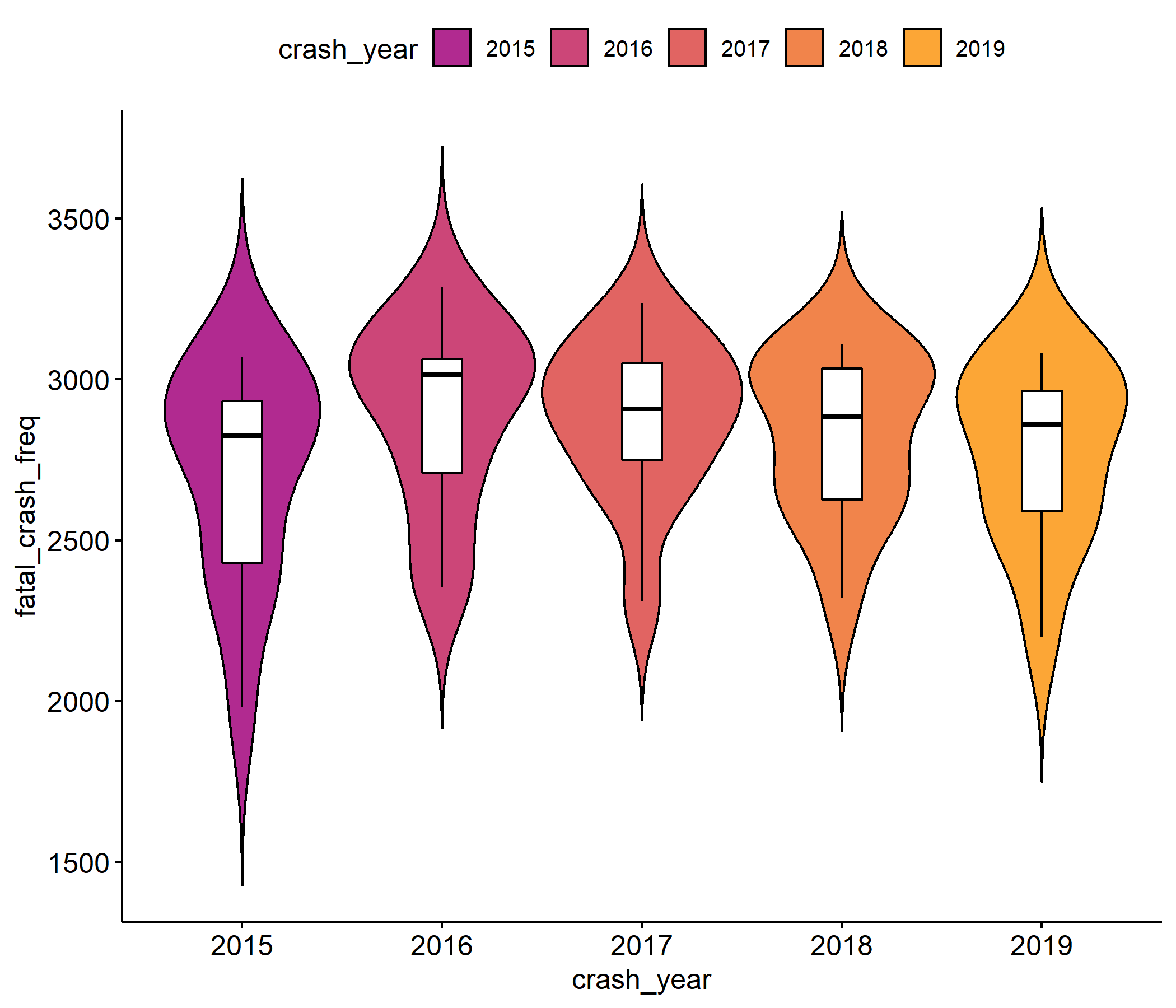
fatal_crash_monthly_counts %>% filter( crash_year %in% c(2015:2019) ) %>% ggviolin( x = "crash_year", y = "fatal_crash_freq", fill = "crash_year", palette = plasma( 5, begin = 0.4, end = 0.8 ), add = "boxplot", add.params = list(fill = "white"), title = paste( "U.S. fatal traffic crash", "distribution by month, 2015–19" ), )
fatal_crash_monthly_counts %>% filter( crash_year %in% c(2015:2019) ) %>% ggviolin( x = "crash_year", y = "fatal_crash_freq", fill = "crash_year", palette = plasma( 5, begin = 0.4, end = 0.8 ), add = "boxplot", add.params = list(fill = "white"), title = paste( "U.S. fatal traffic crash", "distribution by month, 2015–19" ), legend.title = "Crash year", )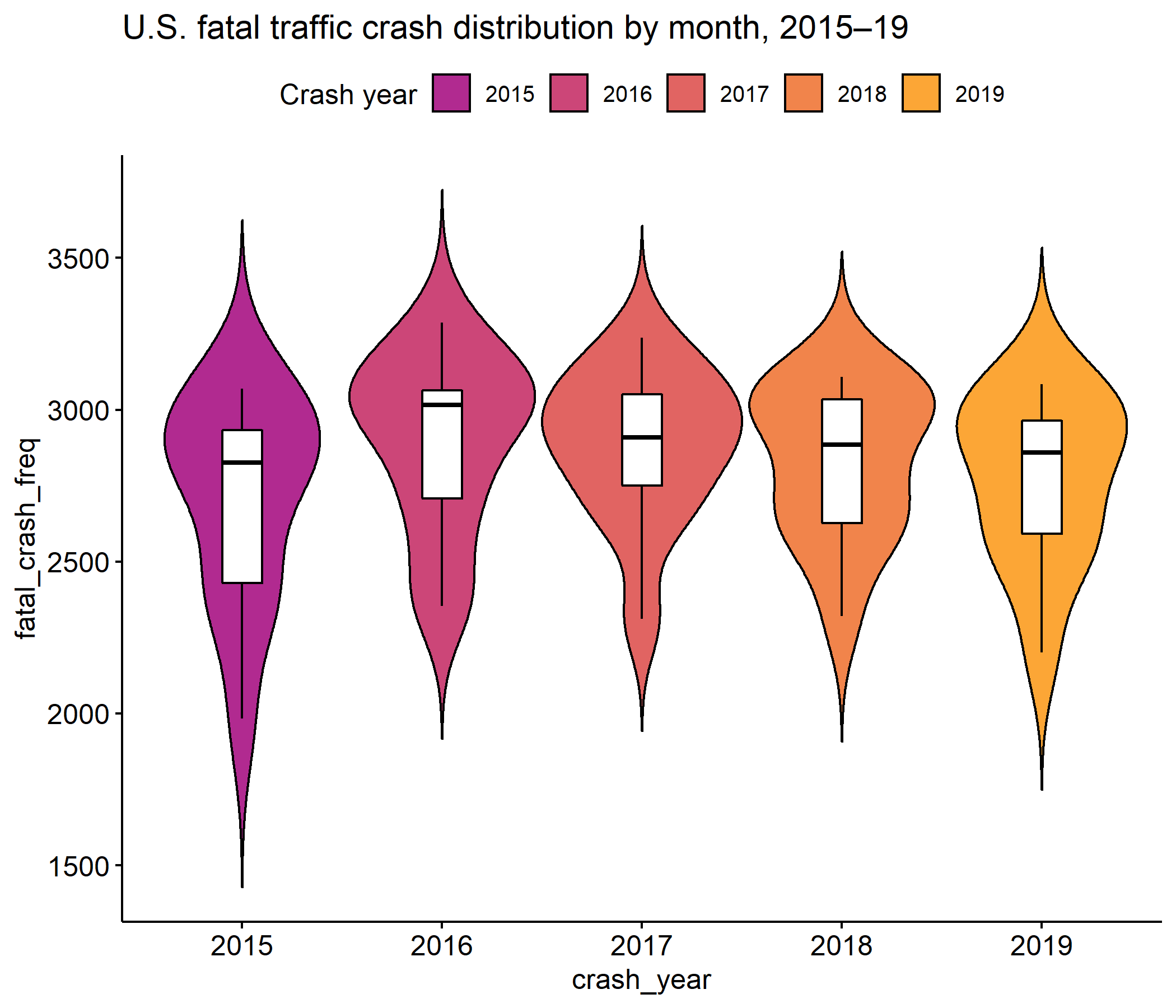
fatal_crash_monthly_counts %>% filter( crash_year %in% c(2015:2019) ) %>% ggviolin( x = "crash_year", y = "fatal_crash_freq", fill = "crash_year", palette = plasma( 5, begin = 0.4, end = 0.8 ), add = "boxplot", add.params = list(fill = "white"), title = paste( "U.S. fatal traffic crash", "distribution by month, 2015–19" ), legend.title = "Crash year", xlab = "", ylab = "" )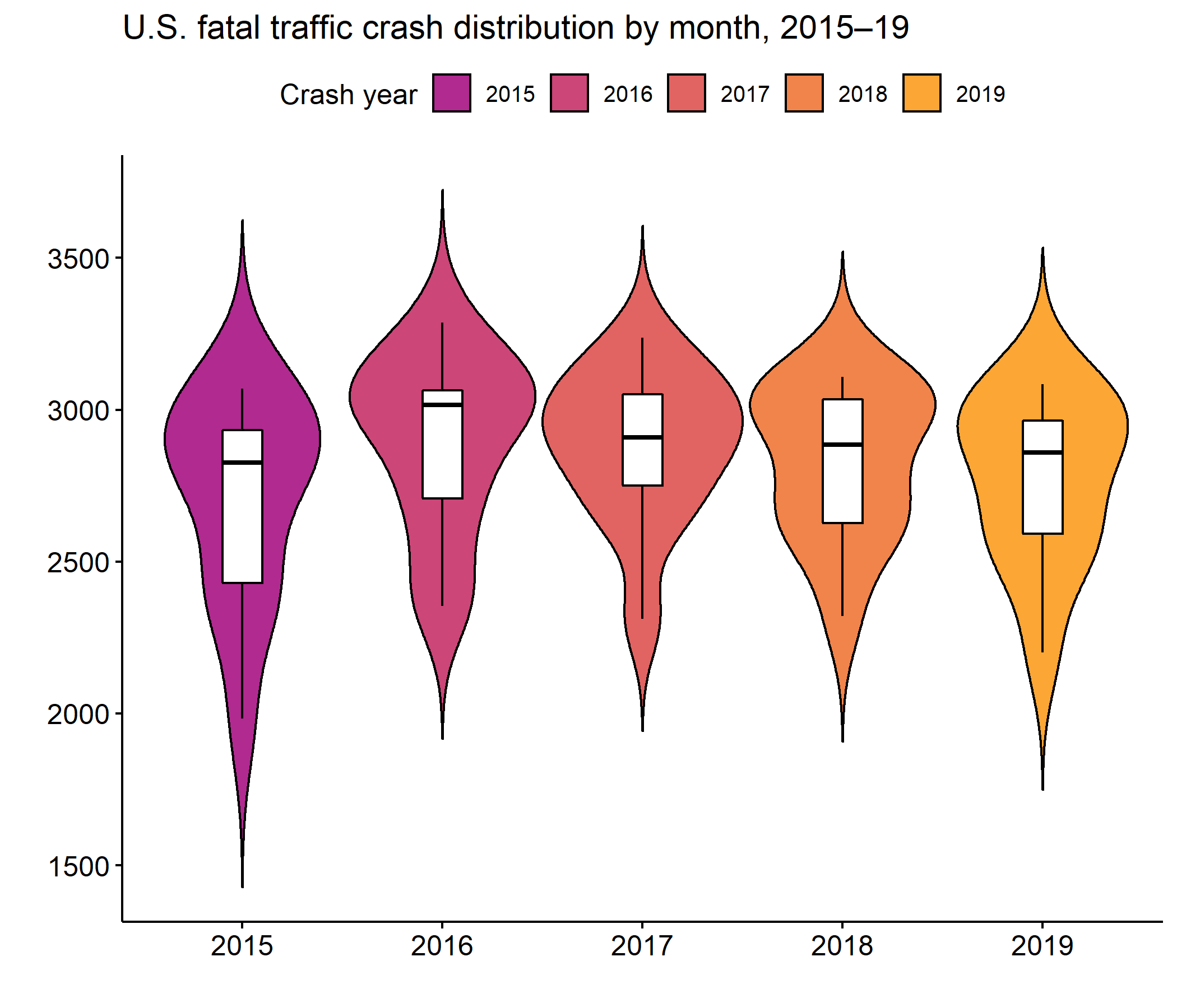
fatal_crash_monthly_counts %>% filter( crash_year %in% c(2015:2019) ) %>% ggviolin( x = "crash_year", y = "fatal_crash_freq", fill = "crash_year", palette = plasma( 5, begin = 0.4, end = 0.8 ), add = "boxplot", add.params = list(fill = "white"), title = paste( "U.S. fatal traffic crash", "distribution by month, 2015–19" ), legend.title = "Crash year", xlab = "", ylab = "" ) + theme_economist()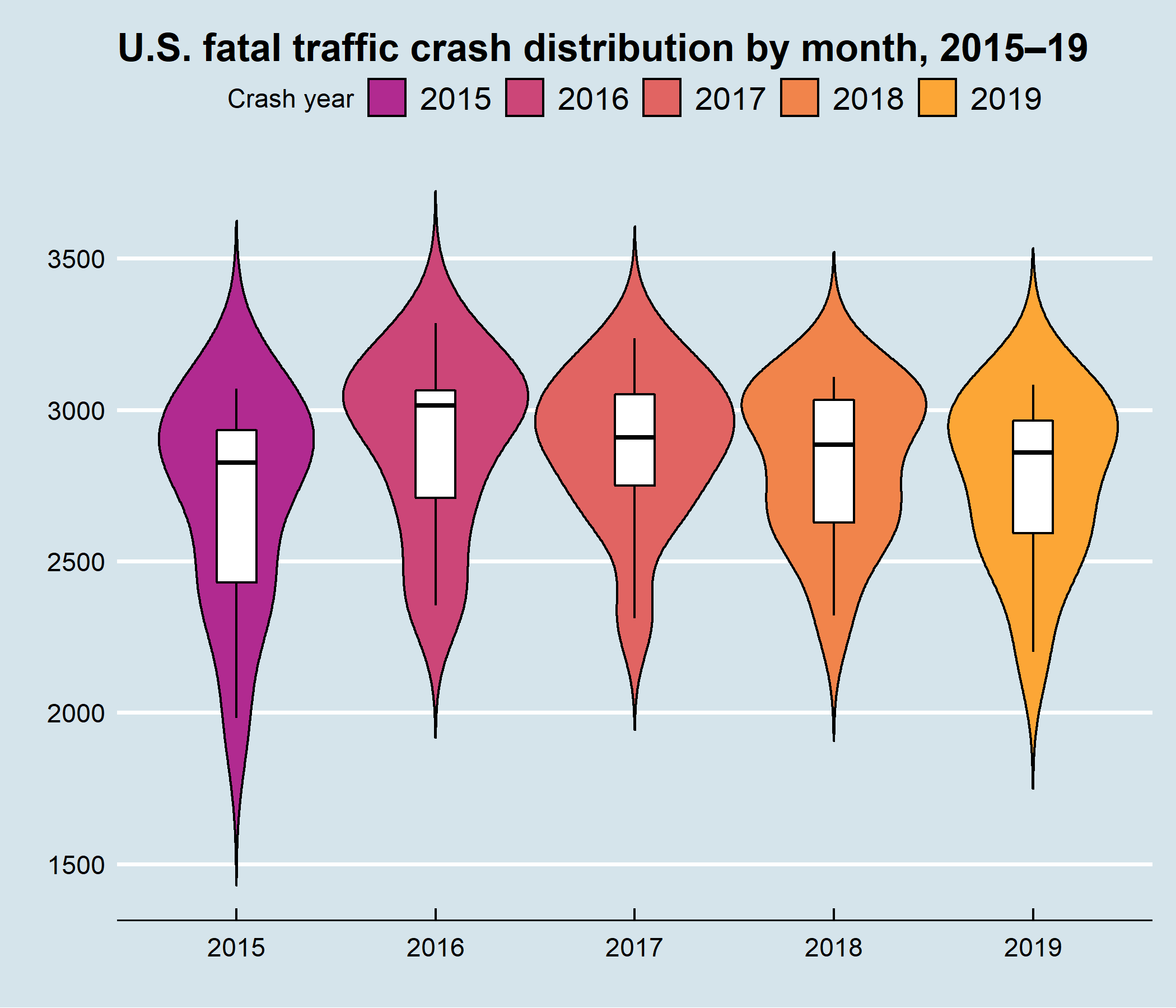
Case for violin plots
The data in each category is shifting overtime, as can clearly be seen in the "Raw" data view, yet the boxplots remain static. Violin plots are a good method for presenting the distribution of a dataset with more detail than is available with a traditional boxplot. This is not to say that using a boxplot is never appropriate, but if you are going to use a boxplot, it is important to make sure the underlying data is distrubuted in a way that important information is not hidden. – Justin Matejka & George Fitzmaurice

Source: Autodesk research
# Create plots for demoggplot()
# Create plots for demoggplot() -> p1ggplot()
# Create plots for demoggplot() -> p1ggplot() + theme_bw()
# Fill a gridp1
# Fill a gridp1 + p2
# Fill a gridp1 + p2 + p1
# Fill a gridp1 + p2 + p1 + p2
# Fill a gridp1 + p2 + p1 + p2 -> ggpatch_grid# Place side-by-sidep1
# Fill a gridp1 + p2 + p1 + p2 -> ggpatch_grid# Place side-by-sidep1 | p2
# Fill a gridp1 + p2 + p1 + p2 -> ggpatch_grid# Place side-by-sidep1 | p2 | p1
# Fill a gridp1 + p2 + p1 + p2 -> ggpatch_grid# Place side-by-sidep1 | p2 | p1 | p2
# Fill a gridp1 + p2 + p1 + p2 -> ggpatch_grid# Place side-by-sidep1 | p2 | p1 | p2 -> ggpatch_juxta# Place on top of each otherp1
# Fill a gridp1 + p2 + p1 + p2 -> ggpatch_grid# Place side-by-sidep1 | p2 | p1 | p2 -> ggpatch_juxta# Place on top of each otherp1 / p2
# Fill a gridp1 + p2 + p1 + p2 -> ggpatch_grid# Place side-by-sidep1 | p2 | p1 | p2 -> ggpatch_juxta# Place on top of each otherp1 / p2 / p1
# Fill a gridp1 + p2 + p1 + p2 -> ggpatch_grid# Place side-by-sidep1 | p2 | p1 | p2 -> ggpatch_juxta# Place on top of each otherp1 / p2 / p1 / p2
# Fill a gridp1 + p2 + p1 + p2 -> ggpatch_grid# Place side-by-sidep1 | p2 | p1 | p2 -> ggpatch_juxta# Place on top of each otherp1 / p2 / p1 / p2 -> ggpatch_updown# Hybrids(p1 / p2)
# Fill a gridp1 + p2 + p1 + p2 -> ggpatch_grid# Place side-by-sidep1 | p2 | p1 | p2 -> ggpatch_juxta# Place on top of each otherp1 / p2 / p1 / p2 -> ggpatch_updown# Hybrids(p1 / p2) | (p1 / p2)
# Fill a gridp1 + p2 + p1 + p2 -> ggpatch_grid# Place side-by-sidep1 | p2 | p1 | p2 -> ggpatch_juxta# Place on top of each otherp1 / p2 / p1 / p2 -> ggpatch_updown# Hybrids(p1 / p2) | (p1 / p2) -> ggpatch_hybrid1(p1 | p2)
# Fill a gridp1 + p2 + p1 + p2 -> ggpatch_grid# Place side-by-sidep1 | p2 | p1 | p2 -> ggpatch_juxta# Place on top of each otherp1 / p2 / p1 / p2 -> ggpatch_updown# Hybrids(p1 / p2) | (p1 / p2) -> ggpatch_hybrid1(p1 | p2) / (p1 | p2)
(p1 | p2) / p1
(p1 | p2) / p1 -> ggpatch_hybrid3p1 | p2
(p1 | p2) / p1 -> ggpatch_hybrid3p1 | p2 | p1 / p2
(p1 | p2) / p1 -> ggpatch_hybrid3p1 | p2 | p1 / p2 -> ggpatch_hybrid4# Asterisk operatorggpatch_hybrid3 * theme_dark()
(p1 | p2) / p1 -> ggpatch_hybrid3p1 | p2 | p1 / p2 -> ggpatch_hybrid4# Asterisk operatorggpatch_hybrid3 * theme_dark() -> ggpatch_star1ggpatch_hybrid4 * theme_dark()
(p1 | p2) / p1 -> ggpatch_hybrid3p1 | p2 | p1 / p2 -> ggpatch_hybrid4# Asterisk operatorggpatch_hybrid3 * theme_dark() -> ggpatch_star1ggpatch_hybrid4 * theme_dark() -> ggpatch_star2# Ampersand operatorggpatch_hybrid3 & theme_dark()
(p1 | p2) / p1 -> ggpatch_hybrid3p1 | p2 | p1 / p2 -> ggpatch_hybrid4# Asterisk operatorggpatch_hybrid3 * theme_dark() -> ggpatch_star1ggpatch_hybrid4 * theme_dark() -> ggpatch_star2# Ampersand operatorggpatch_hybrid3 & theme_dark() -> ggpatch_amp1ggpatch_hybrid4 & theme_dark()
(p1 | p2) / p1 -> ggpatch_hybrid3p1 | p2 | p1 / p2 -> ggpatch_hybrid4# Asterisk operatorggpatch_hybrid3 * theme_dark() -> ggpatch_star1ggpatch_hybrid4 * theme_dark() -> ggpatch_star2# Ampersand operatorggpatch_hybrid3 & theme_dark() -> ggpatch_amp1ggpatch_hybrid4 & theme_dark() -> ggpatch_amp2# Annotationggpatch_amp2
(p1 | p2) / p1 -> ggpatch_hybrid3p1 | p2 | p1 / p2 -> ggpatch_hybrid4# Asterisk operatorggpatch_hybrid3 * theme_dark() -> ggpatch_star1ggpatch_hybrid4 * theme_dark() -> ggpatch_star2# Ampersand operatorggpatch_hybrid3 & theme_dark() -> ggpatch_amp1ggpatch_hybrid4 & theme_dark() -> ggpatch_amp2# Annotationggpatch_amp2 + plot_annotation(tag_levels = "A")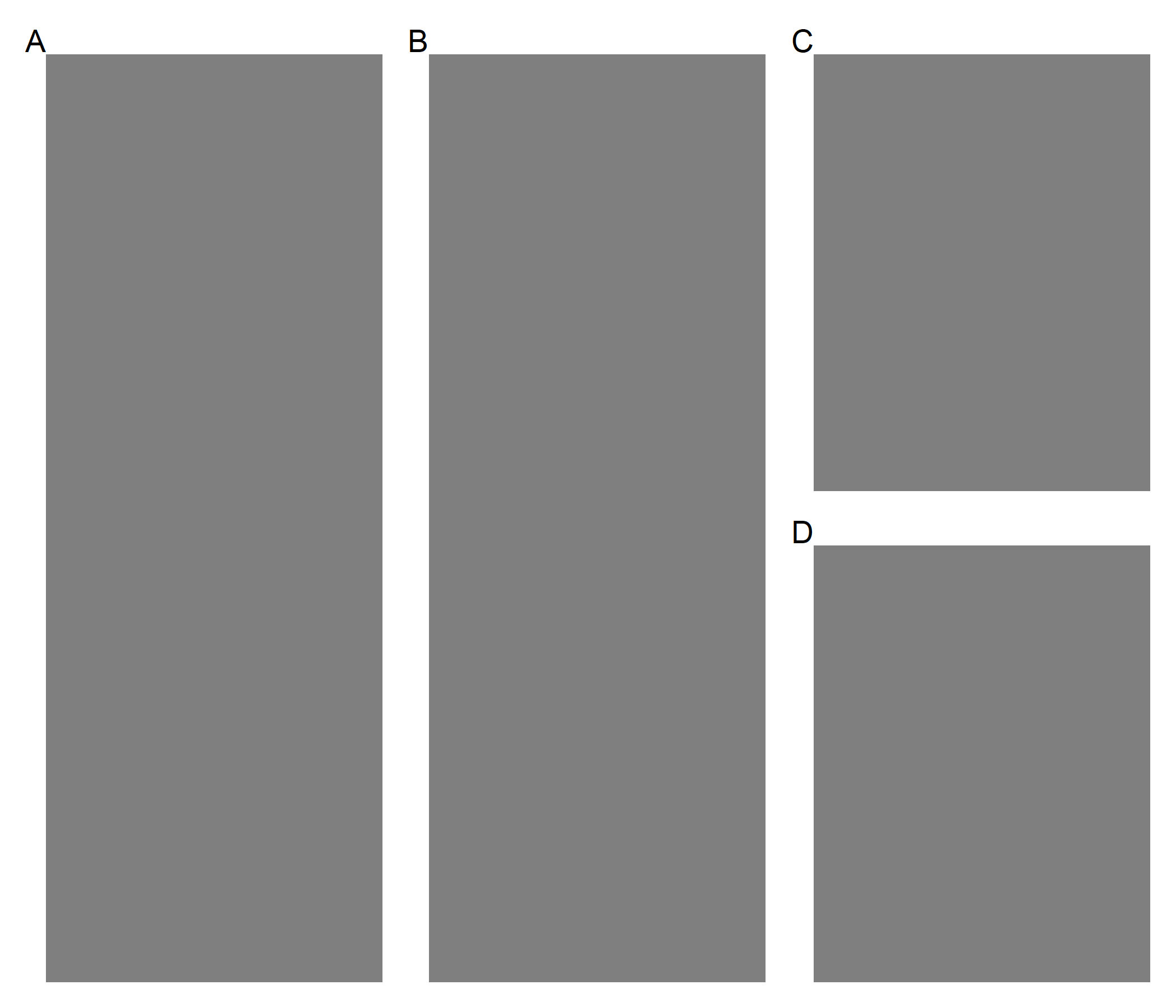
(p1 | p2) / p1 -> ggpatch_hybrid3p1 | p2 | p1 / p2 -> ggpatch_hybrid4# Asterisk operatorggpatch_hybrid3 * theme_dark() -> ggpatch_star1ggpatch_hybrid4 * theme_dark() -> ggpatch_star2# Ampersand operatorggpatch_hybrid3 & theme_dark() -> ggpatch_amp1ggpatch_hybrid4 & theme_dark() -> ggpatch_amp2# Annotationggpatch_amp2 + plot_annotation(tag_levels = "A") -> ggpatch_annot1ggpatch_amp2[[3]] <- ggpatch_amp2[[3]] + plot_layout(tag_level = "new")ggpatch_amp2
(p1 | p2) / p1 -> ggpatch_hybrid3p1 | p2 | p1 / p2 -> ggpatch_hybrid4# Asterisk operatorggpatch_hybrid3 * theme_dark() -> ggpatch_star1ggpatch_hybrid4 * theme_dark() -> ggpatch_star2# Ampersand operatorggpatch_hybrid3 & theme_dark() -> ggpatch_amp1ggpatch_hybrid4 & theme_dark() -> ggpatch_amp2# Annotationggpatch_amp2 + plot_annotation(tag_levels = "A") -> ggpatch_annot1ggpatch_amp2[[3]] <- ggpatch_amp2[[3]] + plot_layout(tag_level = "new")ggpatch_amp2 + plot_annotation( tag_levels = c("A", "1") )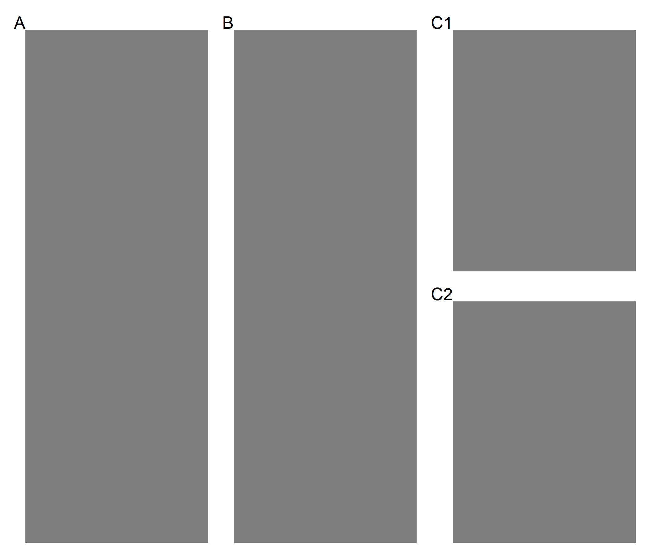
(lol_chart / dev_chart)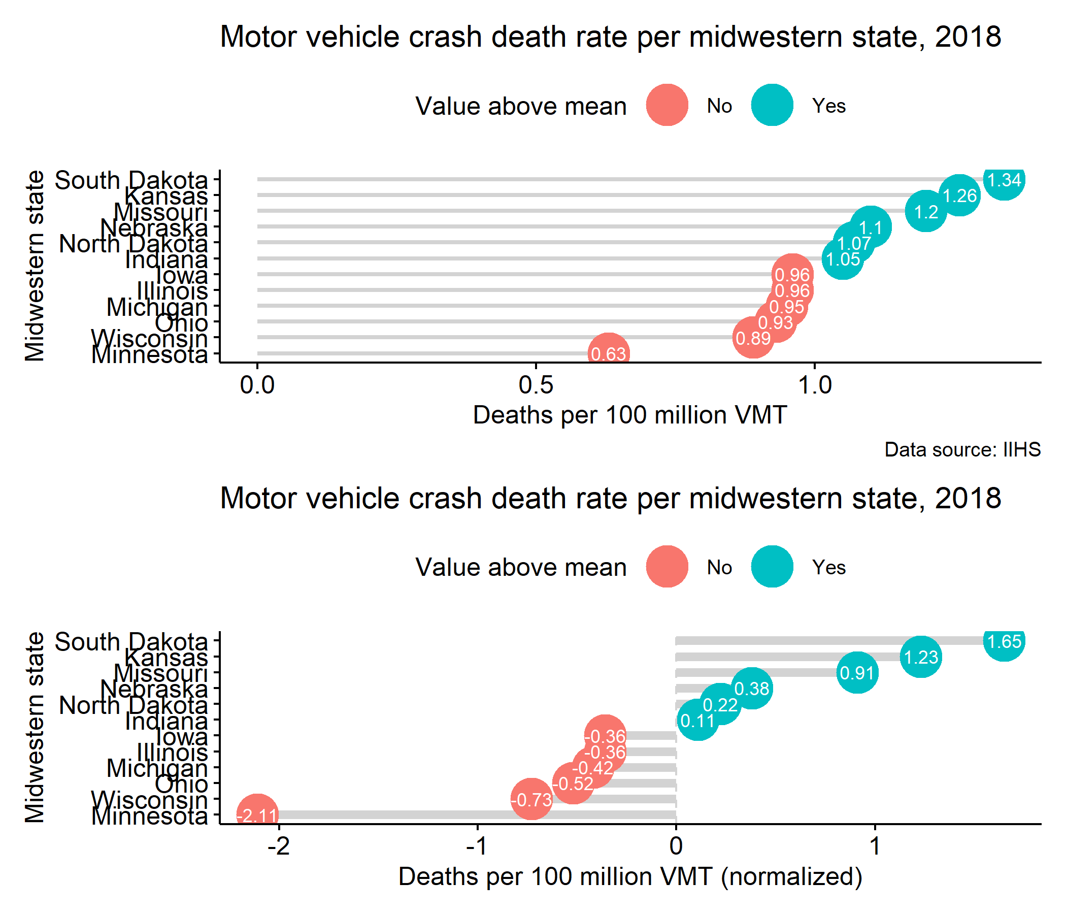
(lol_chart / dev_chart) -> ggpatch_finalggpatch_final[[1]]
(lol_chart / dev_chart) -> ggpatch_finalggpatch_final[[1]] + labs(title = NULL, caption = NULL)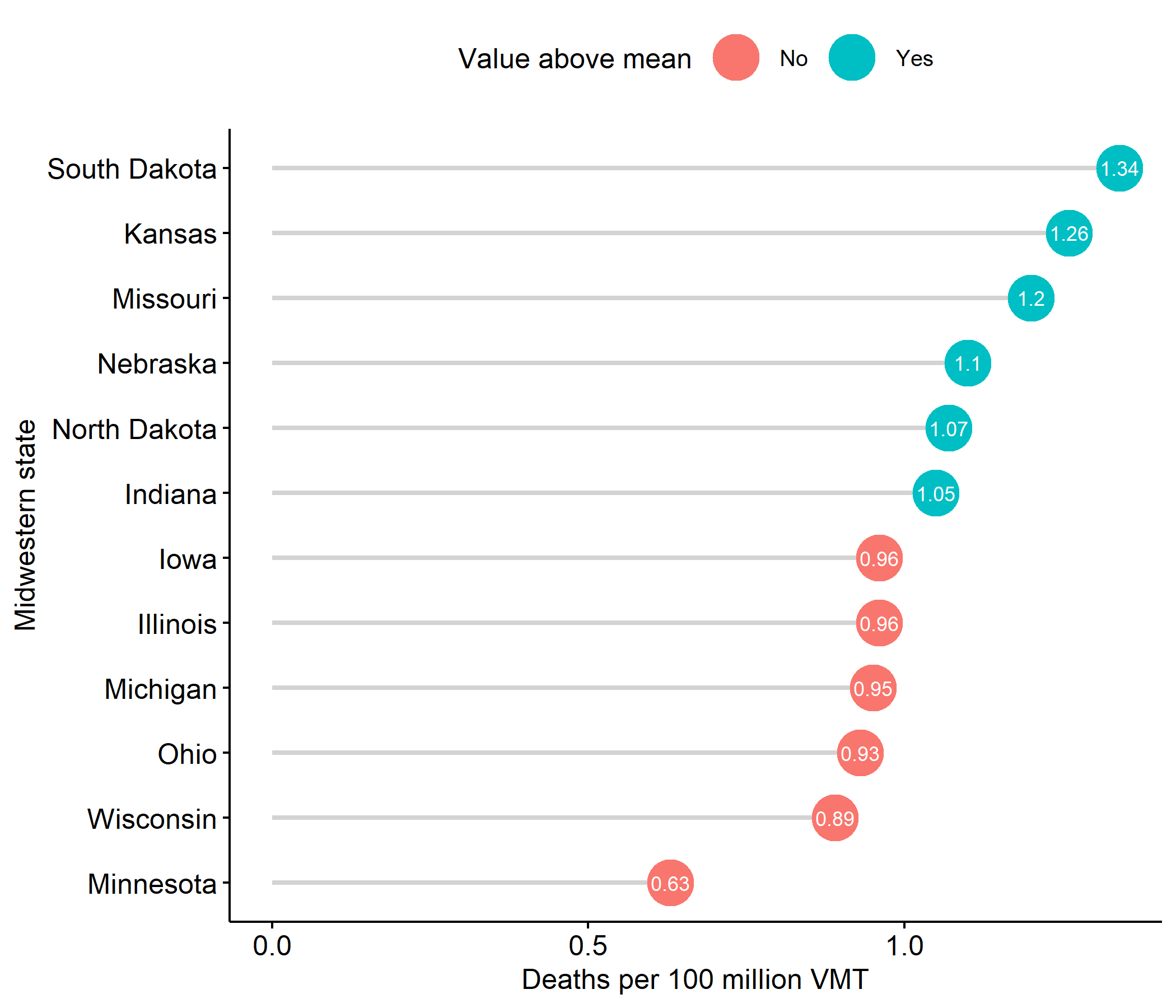
(lol_chart / dev_chart) -> ggpatch_finalggpatch_final[[1]] + labs(title = NULL, caption = NULL) -> ggpatch_final[[1]]ggpatch_final[[2]]
(lol_chart / dev_chart) -> ggpatch_finalggpatch_final[[1]] + labs(title = NULL, caption = NULL) -> ggpatch_final[[1]]ggpatch_final[[2]] + labs(title = NULL)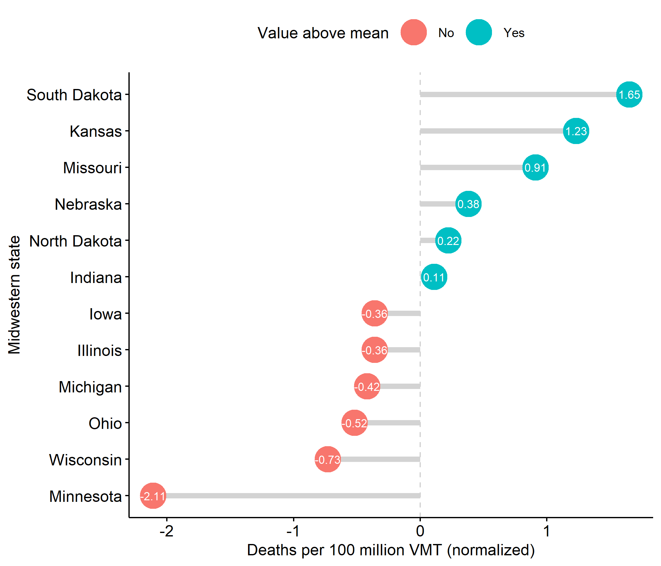
(lol_chart / dev_chart) -> ggpatch_finalggpatch_final[[1]] + labs(title = NULL, caption = NULL) -> ggpatch_final[[1]]ggpatch_final[[2]] + labs(title = NULL) -> ggpatch_final[[2]]ggpatch_final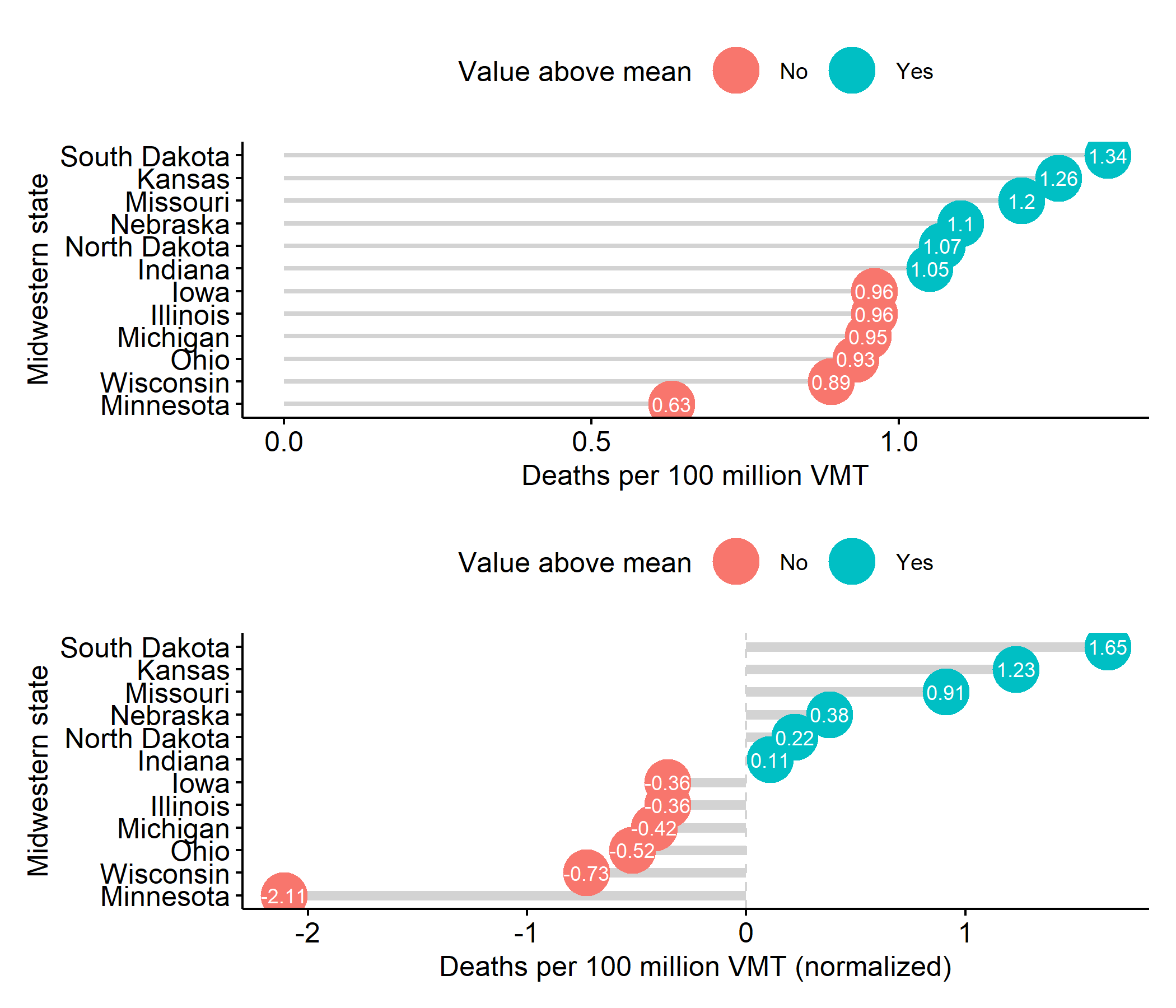
(lol_chart / dev_chart) -> ggpatch_finalggpatch_final[[1]] + labs(title = NULL, caption = NULL) -> ggpatch_final[[1]]ggpatch_final[[2]] + labs(title = NULL) -> ggpatch_final[[2]]ggpatch_final + plot_layout(guides = "collect")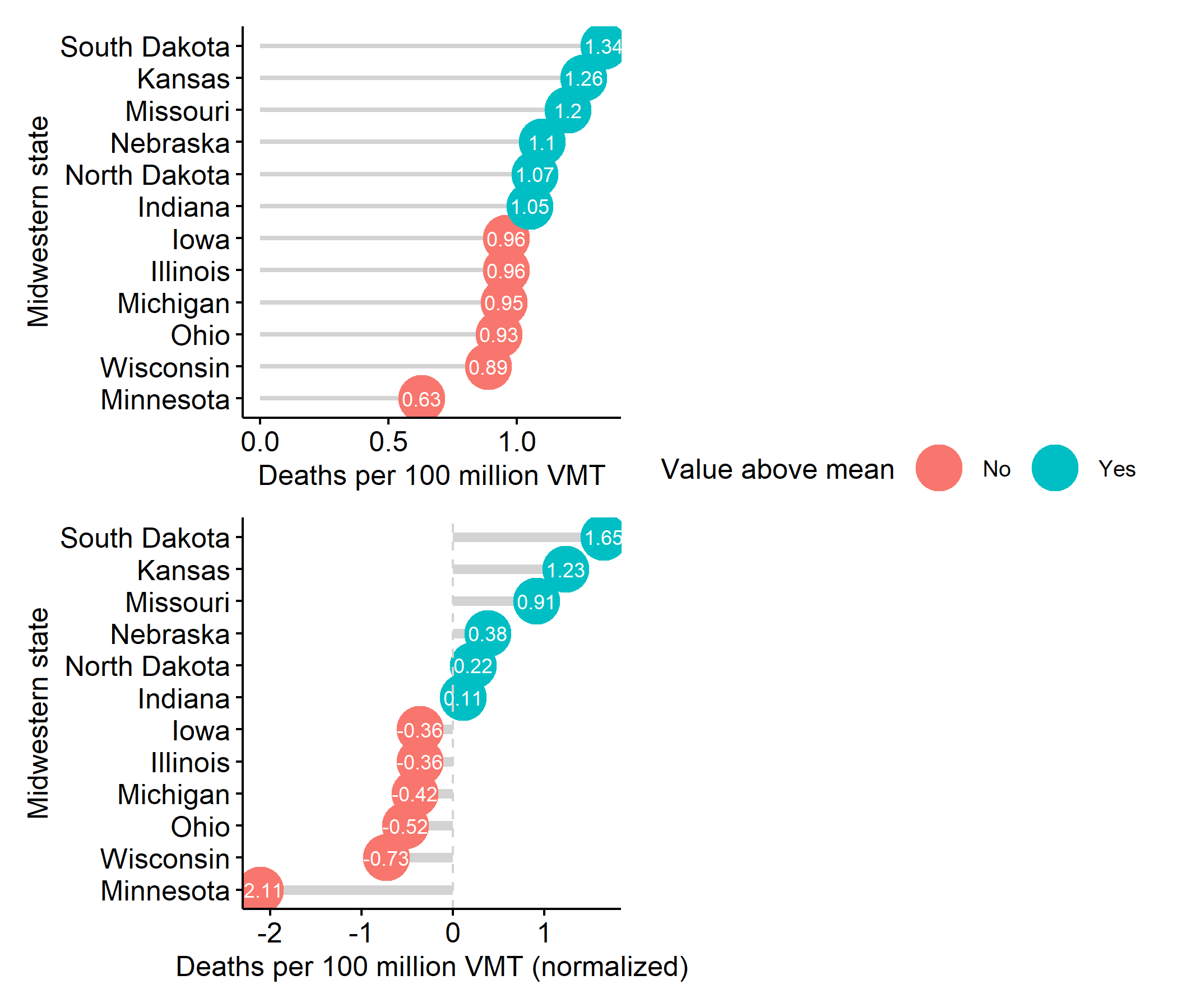
(lol_chart / dev_chart) -> ggpatch_finalggpatch_final[[1]] + labs(title = NULL, caption = NULL) -> ggpatch_final[[1]]ggpatch_final[[2]] + labs(title = NULL) -> ggpatch_final[[2]]ggpatch_final + plot_layout(guides = "collect") + plot_annotation( title = paste( "Motor vehicle crash death rate", "per midwestern state, 2018" ), caption = "Data source: IIHS", theme = theme_pubr(), tag_levels = "A", tag_prefix = "Fig. " )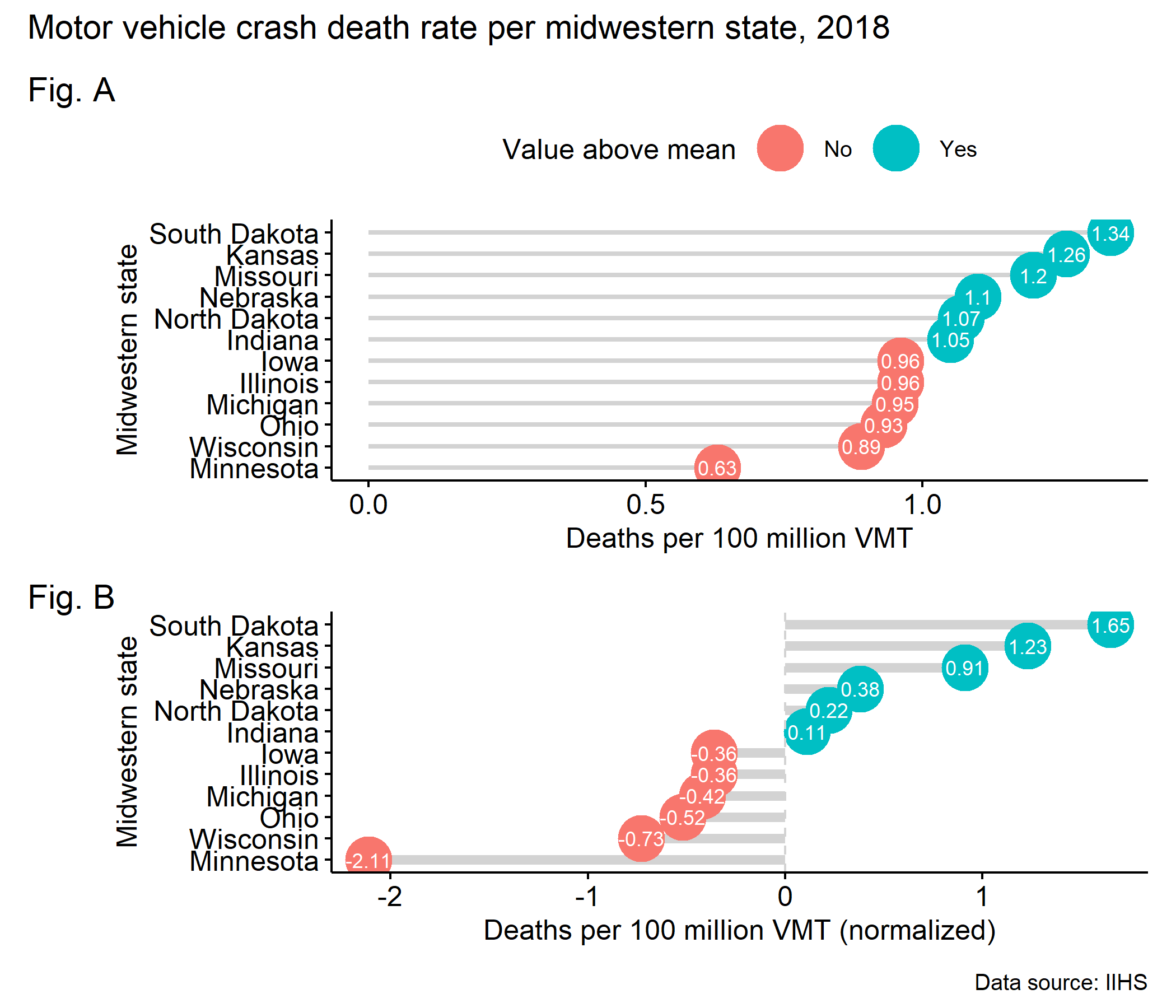
(lol_chart / dev_chart) -> ggpatch_finalggpatch_final[[1]] + labs(title = NULL, caption = NULL) -> ggpatch_final[[1]]ggpatch_final[[2]] + labs(title = NULL) -> ggpatch_final[[2]]ggpatch_final + plot_layout(guides = "collect") + plot_annotation( title = paste( "Motor vehicle crash death rate", "per midwestern state, 2018" ), caption = "Data source: IIHS", theme = theme_pubr(), tag_levels = "A", tag_prefix = "Fig. " ) & theme( plot.tag = element_text(size = 10) )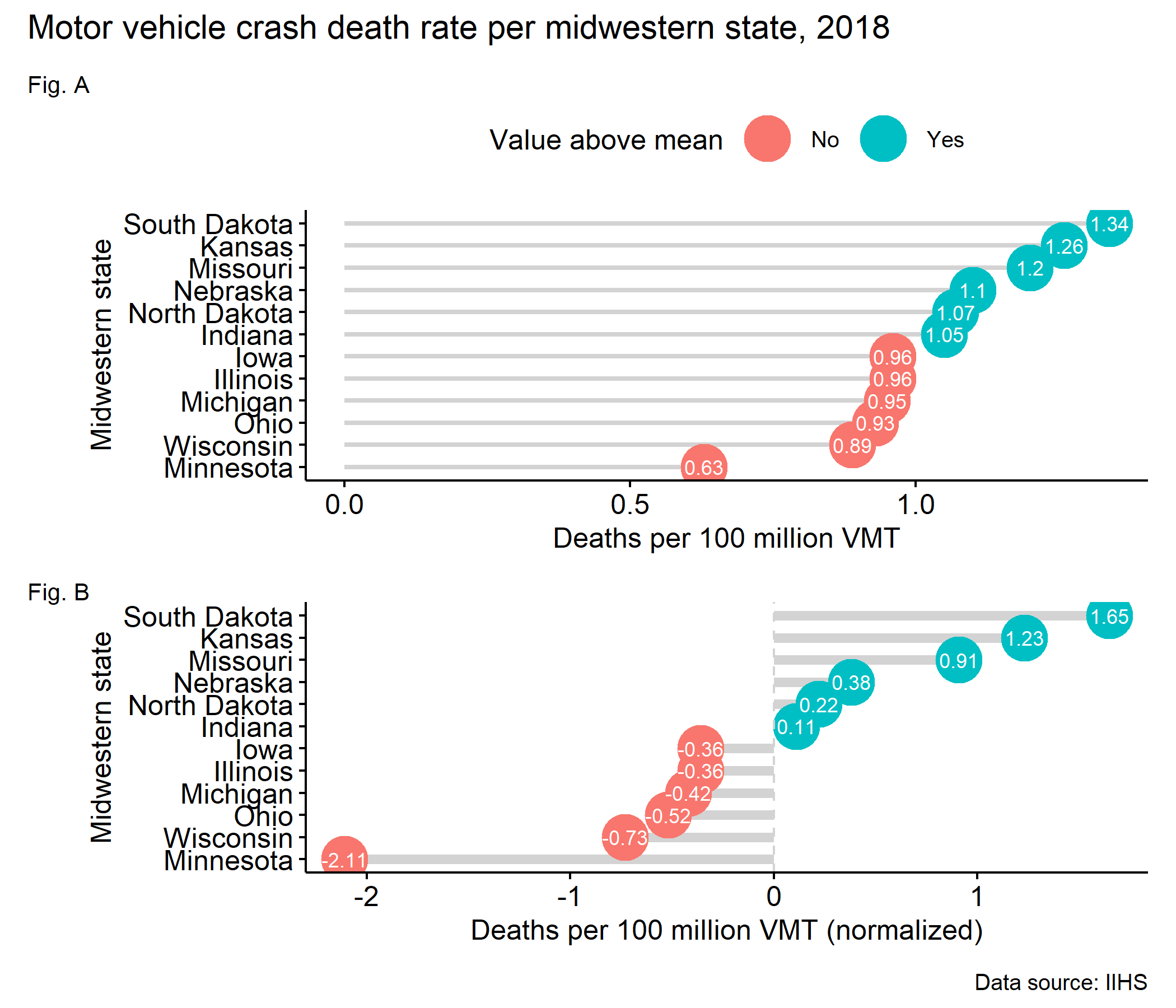
(lol_chart / dev_chart) -> ggpatch_finalggpatch_final[[1]] + labs(title = NULL, caption = NULL) -> ggpatch_final[[1]]ggpatch_final[[2]] + labs(title = NULL) -> ggpatch_final[[2]]ggpatch_final + plot_layout(guides = "collect") + plot_annotation( )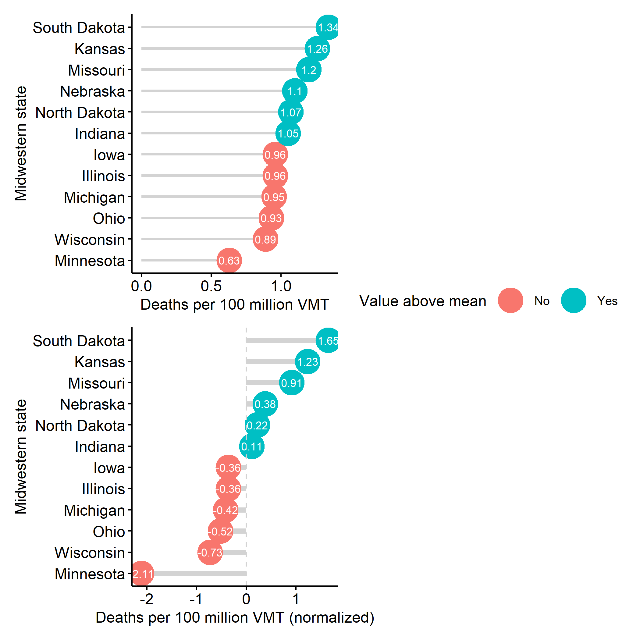
(lol_chart / dev_chart) -> ggpatch_finalggpatch_final[[1]] + labs(title = NULL, caption = NULL) -> ggpatch_final[[1]]ggpatch_final[[2]] + labs(title = NULL) -> ggpatch_final[[2]]ggpatch_final + plot_layout(guides = "collect") + plot_annotation( title = paste( "Motor vehicle crash death rate", "per midwestern state, 2018" ), )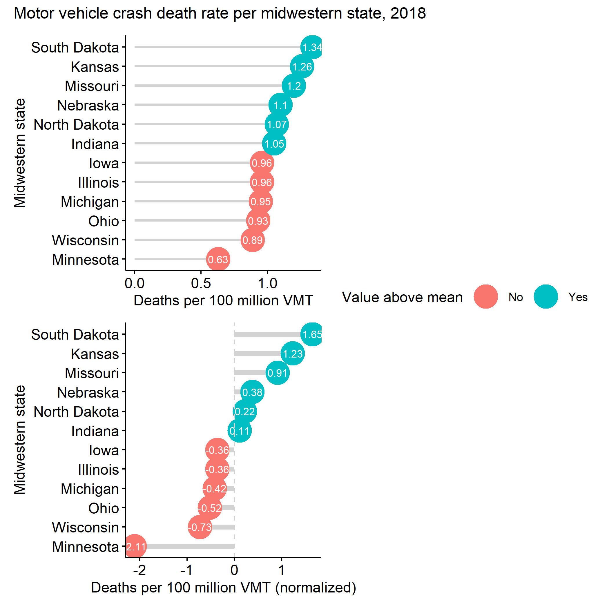
(lol_chart / dev_chart) -> ggpatch_finalggpatch_final[[1]] + labs(title = NULL, caption = NULL) -> ggpatch_final[[1]]ggpatch_final[[2]] + labs(title = NULL) -> ggpatch_final[[2]]ggpatch_final + plot_layout(guides = "collect") + plot_annotation( title = paste( "Motor vehicle crash death rate", "per midwestern state, 2018" ), caption = "Data source: IIHS", )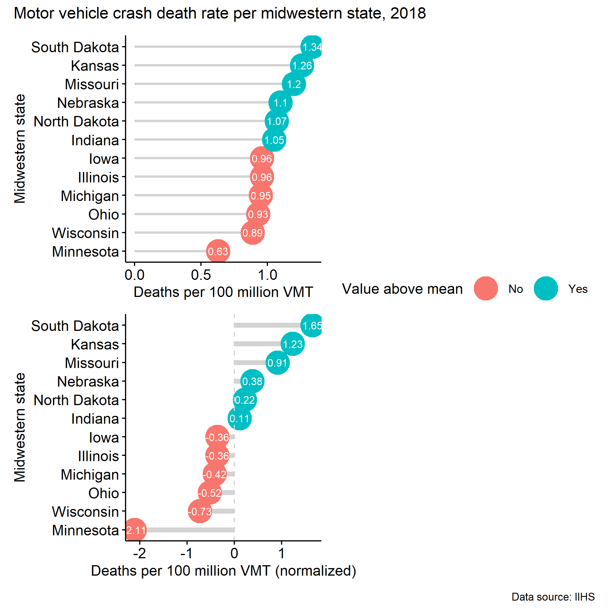
(lol_chart / dev_chart) -> ggpatch_finalggpatch_final[[1]] + labs(title = NULL, caption = NULL) -> ggpatch_final[[1]]ggpatch_final[[2]] + labs(title = NULL) -> ggpatch_final[[2]]ggpatch_final + plot_layout(guides = "collect") + plot_annotation( title = paste( "Motor vehicle crash death rate", "per midwestern state, 2018" ), caption = "Data source: IIHS", theme = theme_pubr(), )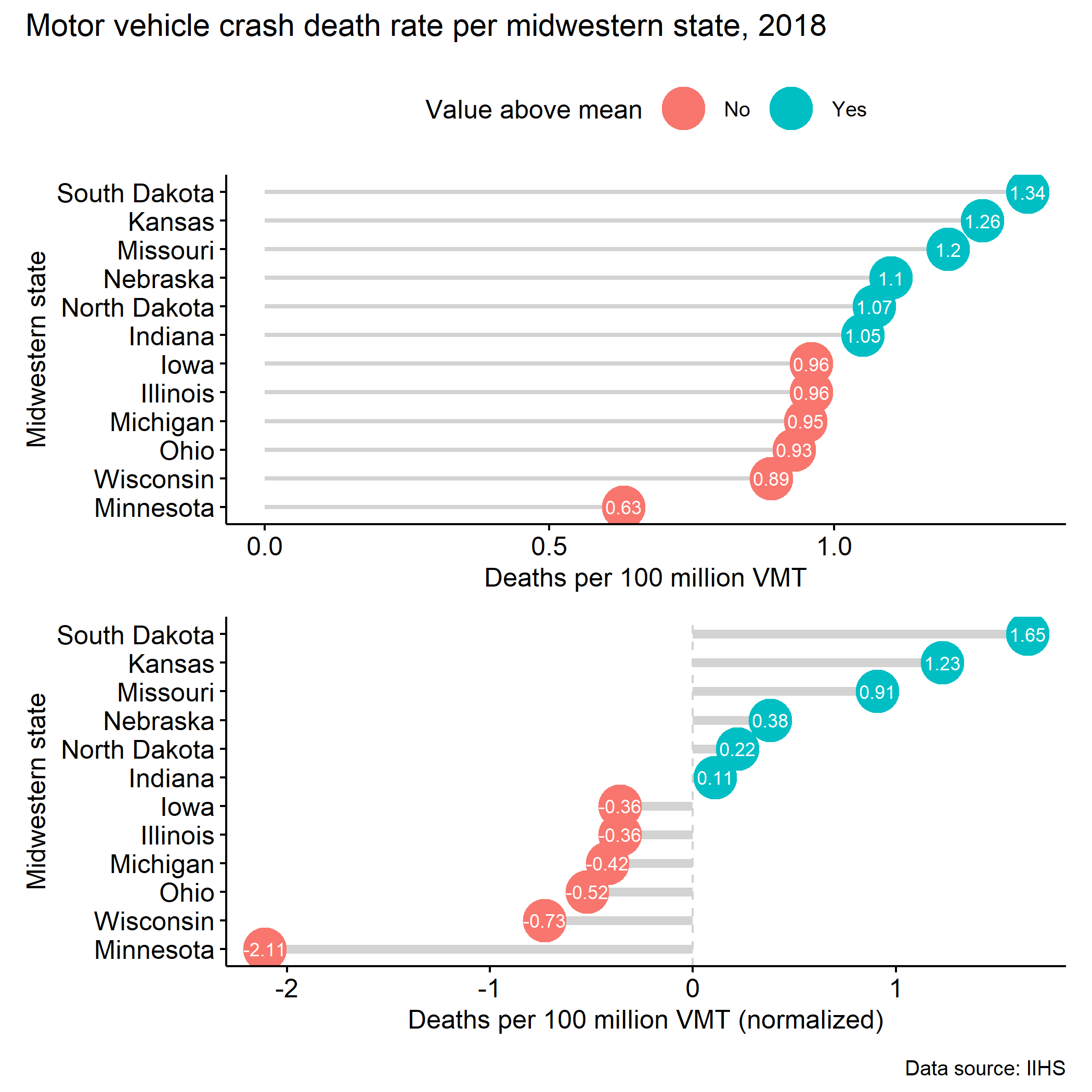
(lol_chart / dev_chart) -> ggpatch_finalggpatch_final[[1]] + labs(title = NULL, caption = NULL) -> ggpatch_final[[1]]ggpatch_final[[2]] + labs(title = NULL) -> ggpatch_final[[2]]ggpatch_final + plot_layout(guides = "collect") + plot_annotation( title = paste( "Motor vehicle crash death rate", "per midwestern state, 2018" ), caption = "Data source: IIHS", theme = theme_pubr(), tag_levels = "A", )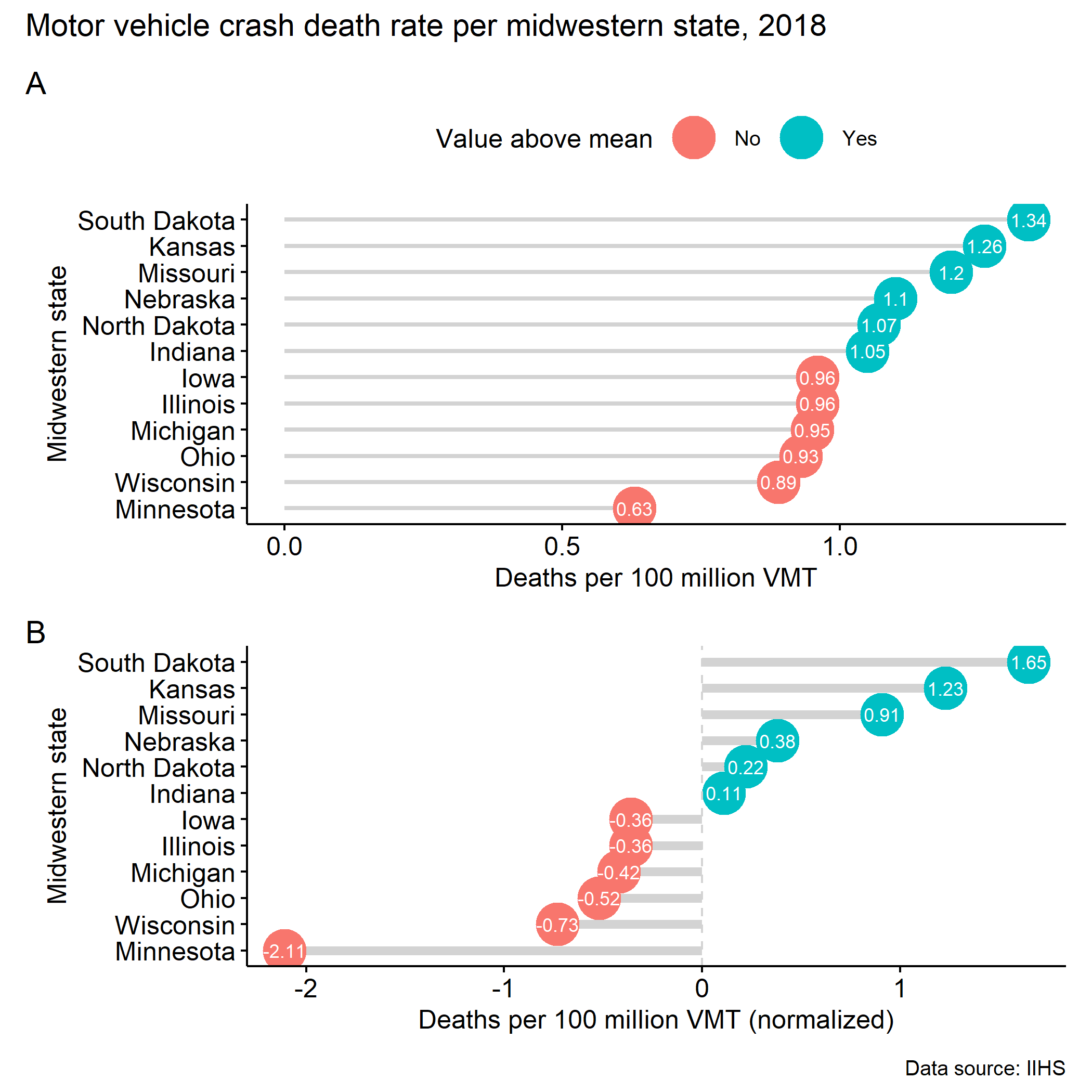
(lol_chart / dev_chart) -> ggpatch_finalggpatch_final[[1]] + labs(title = NULL, caption = NULL) -> ggpatch_final[[1]]ggpatch_final[[2]] + labs(title = NULL) -> ggpatch_final[[2]]ggpatch_final + plot_layout(guides = "collect") + plot_annotation( title = paste( "Motor vehicle crash death rate", "per midwestern state, 2018" ), caption = "Data source: IIHS", theme = theme_pubr(), tag_levels = "A", tag_prefix = "Fig. " )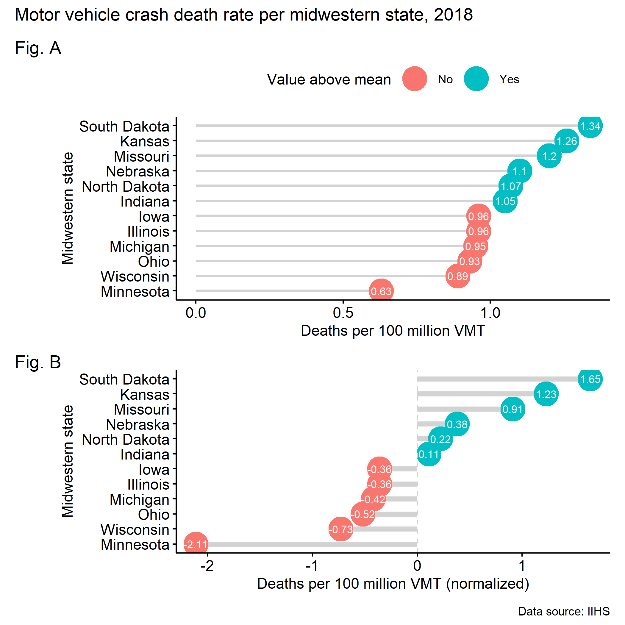
(lol_chart / dev_chart) -> ggpatch_finalggpatch_final[[1]] + labs(title = NULL, caption = NULL) -> ggpatch_final[[1]]ggpatch_final[[2]] + labs(title = NULL) -> ggpatch_final[[2]]ggpatch_final + plot_layout(guides = "collect") + plot_annotation( title = paste( "Motor vehicle crash death rate", "per midwestern state, 2018" ), caption = "Data source: IIHS", theme = theme_pubr(), tag_levels = "A", tag_prefix = "Fig. " ) & theme( plot.tag = element_text(size = 10) )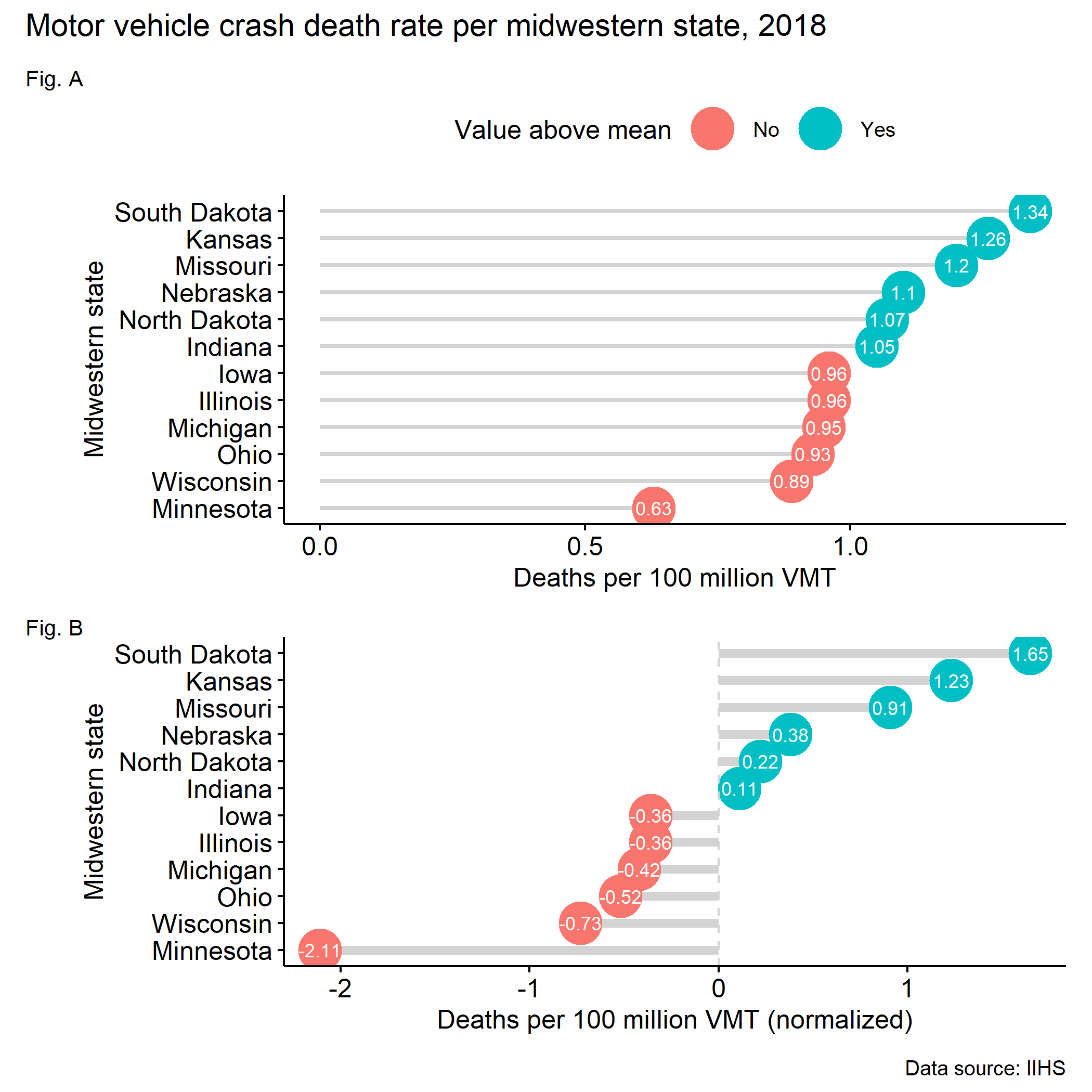
ggdumb_df %>% ggplot()
ggdumb_df %>% ggplot() + aes( y = state, x = prop_2017, xend = prop_2018 )
ggdumb_df %>% ggplot() + aes( y = state, x = prop_2017, xend = prop_2018 ) + geom_dumbbell( size = 1.5, color = "#b2b2b2", size_x = 3, colour_x = "#9fb059", size_xend = 3, colour_xend = "#edae52" )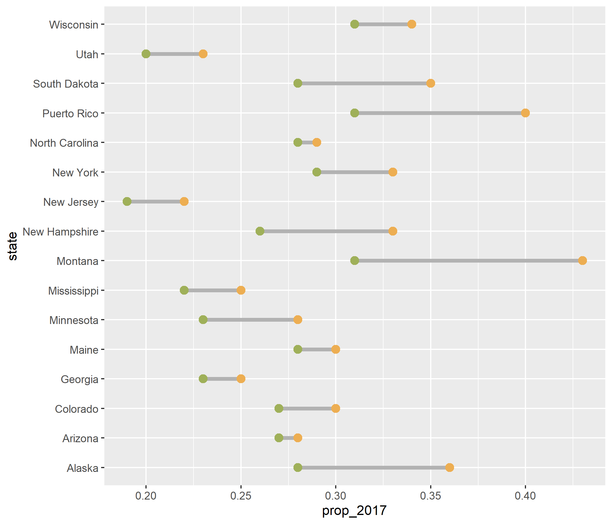
ggdumb_df %>% ggplot() + aes( y = state, x = prop_2017, xend = prop_2018 ) + geom_dumbbell( size = 1.5, color = "#b2b2b2", size_x = 3, colour_x = "#9fb059", size_xend = 3, colour_xend = "#edae52" ) + aes(y = fct_reorder(state, diff))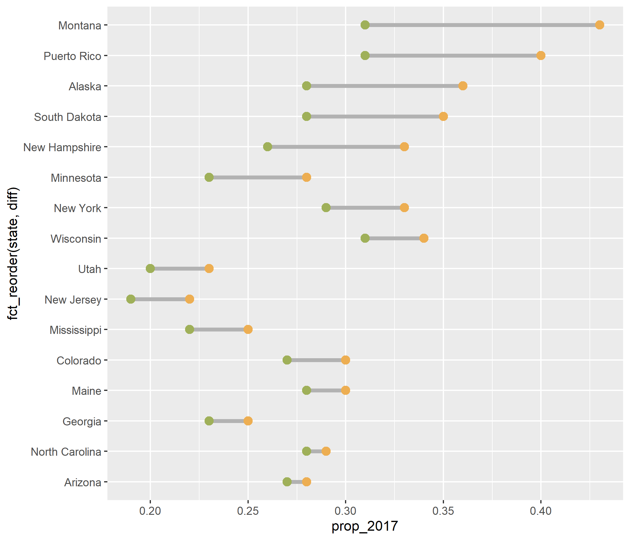
ggdumb_df %>% ggplot() + aes( y = state, x = prop_2017, xend = prop_2018 ) + geom_dumbbell( size = 1.5, color = "#b2b2b2", size_x = 3, colour_x = "#9fb059", size_xend = 3, colour_xend = "#edae52" ) + aes(y = fct_reorder(state, diff)) + geom_text( data = filter( ggdumb_df, state == "Montana" ), aes( x = prop_2017, y = state, label = "Year 2017" ), color = "#9fb059", size = 3, vjust = -2, fontface = "bold" )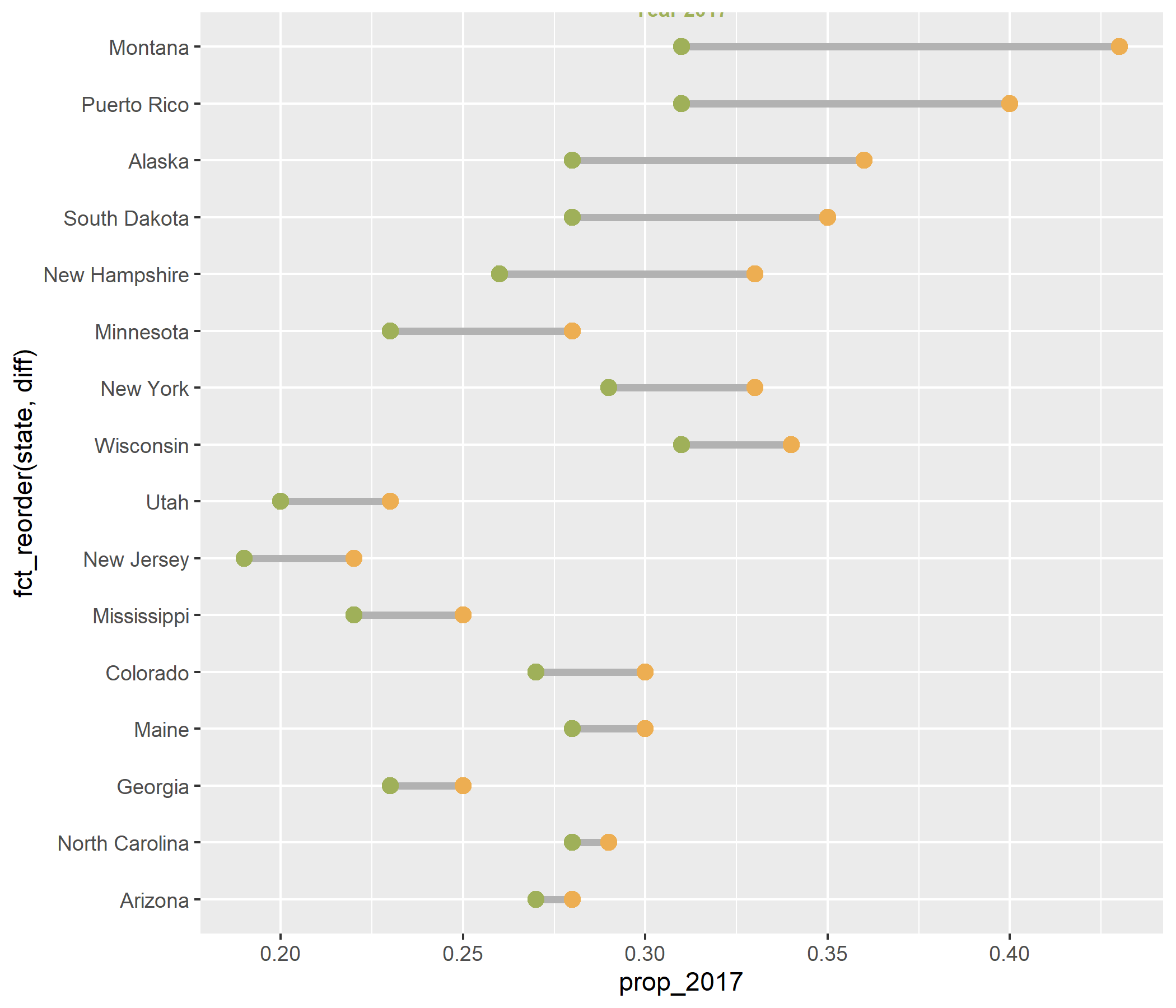
ggdumb_part1
ggdumb_part1 + geom_text( data = filter( ggdumb_df, state == "Montana" ), aes( x = prop_2018, y = state, label = "Year 2018" ), color = "#edae52", size = 3, vjust = -2, fontface = "bold" )
ggdumb_part1 + geom_text( data = filter( ggdumb_df, state == "Montana" ), aes( x = prop_2018, y = state, label = "Year 2018" ), color = "#edae52", size = 3, vjust = -2, fontface = "bold" ) + scale_y_discrete( expand = expansion(0, 1.2) )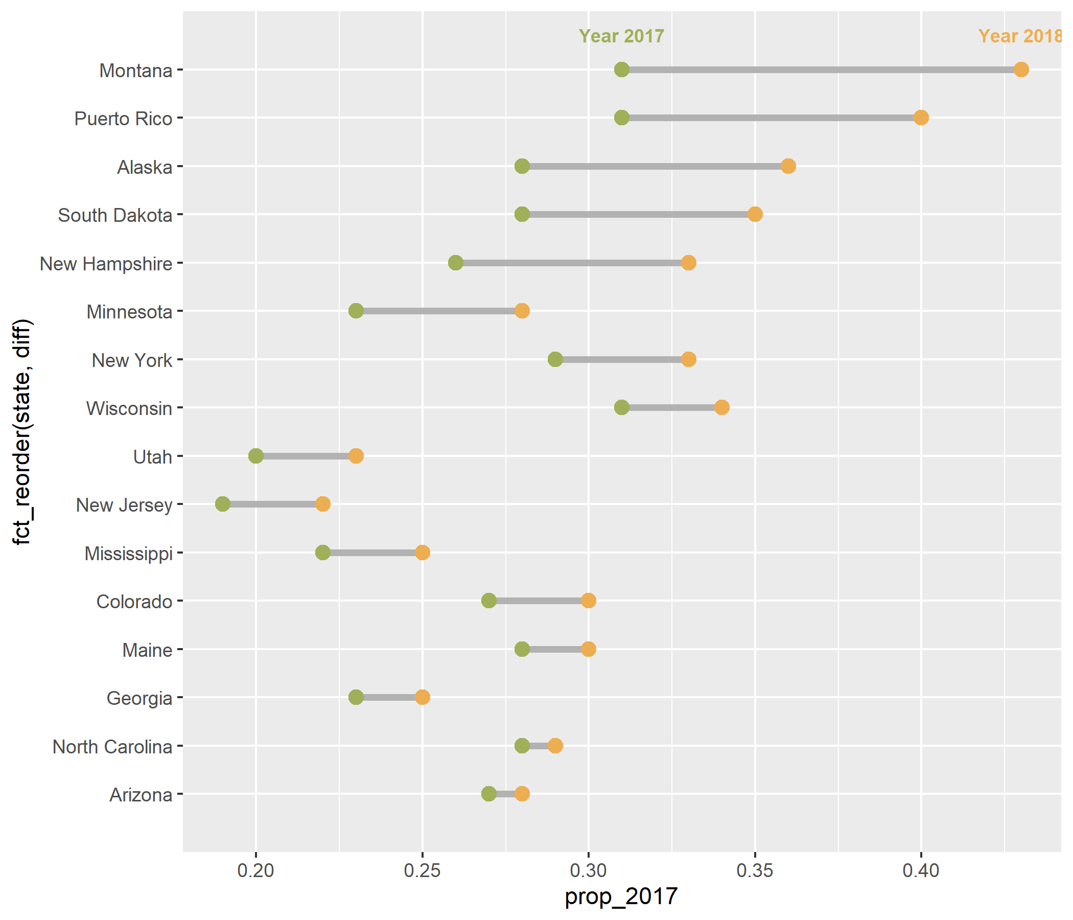
ggdumb_part1 + geom_text( data = filter( ggdumb_df, state == "Montana" ), aes( x = prop_2018, y = state, label = "Year 2018" ), color = "#edae52", size = 3, vjust = -2, fontface = "bold" ) + scale_y_discrete( expand = expansion(0, 1.2) ) + geom_text( aes(x = prop_2017, y = state, label = lab_2017), color = "#9fb059", size = 2.75, vjust = 2.5 )
ggdumb_part1 + geom_text( data = filter( ggdumb_df, state == "Montana" ), aes( x = prop_2018, y = state, label = "Year 2018" ), color = "#edae52", size = 3, vjust = -2, fontface = "bold" ) + scale_y_discrete( expand = expansion(0, 1.2) ) + geom_text( aes(x = prop_2017, y = state, label = lab_2017), color = "#9fb059", size = 2.75, vjust = 2.5 ) + geom_text( aes(x = prop_2018, y = state, label = lab_2018), color = "#edae52", size = 2.75, vjust = 2.5 )
ggdumb_part2
ggdumb_part2 + geom_rect( aes( xmin = 0.55, xmax = 0.675, ymin = -Inf, ymax = Inf ), fill = "#efefe3" )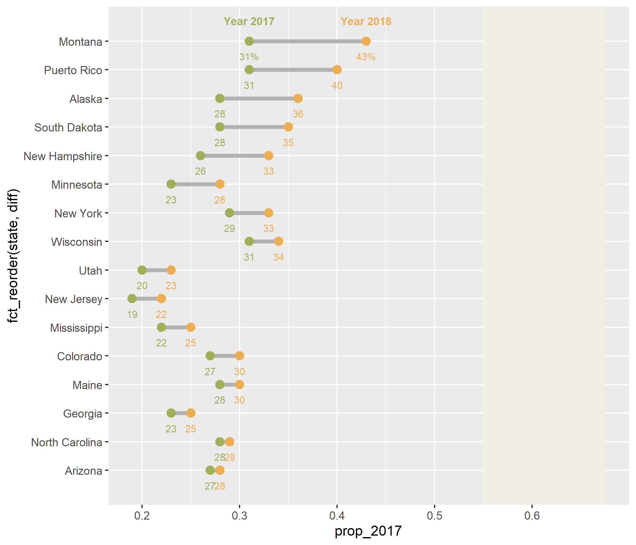
ggdumb_part2 + geom_rect( aes( xmin = 0.55, xmax = 0.675, ymin = -Inf, ymax = Inf ), fill = "#efefe3" ) + geom_text( aes( y = state, x = 0.6125, label = diff_pretty, ), fontface = "bold", size = 3 )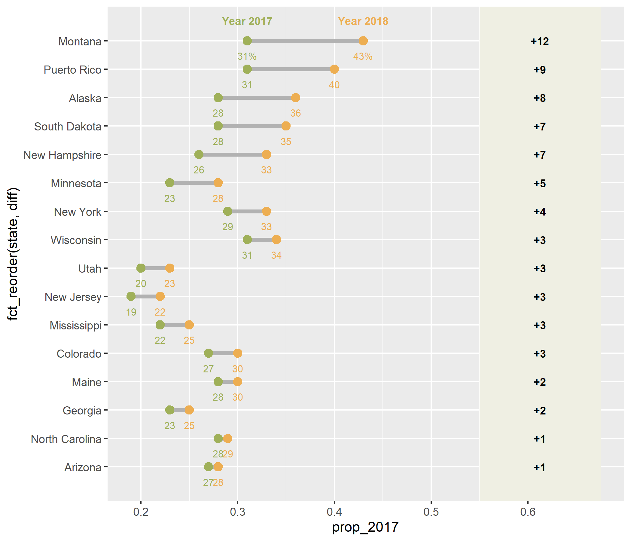
ggdumb_part2 + geom_rect( aes( xmin = 0.55, xmax = 0.675, ymin = -Inf, ymax = Inf ), fill = "#efefe3" ) + geom_text( aes( y = state, x = 0.6125, label = diff_pretty, ), fontface = "bold", size = 3 ) + geom_text( data = filter( ggdumb_df, state == "Montana" ), aes( x = 0.6125, y = state, label = "DIFF" ), color = "#7a7d7e", size = 3.1, vjust = -2, fontface = "bold" )
ggdumb_part3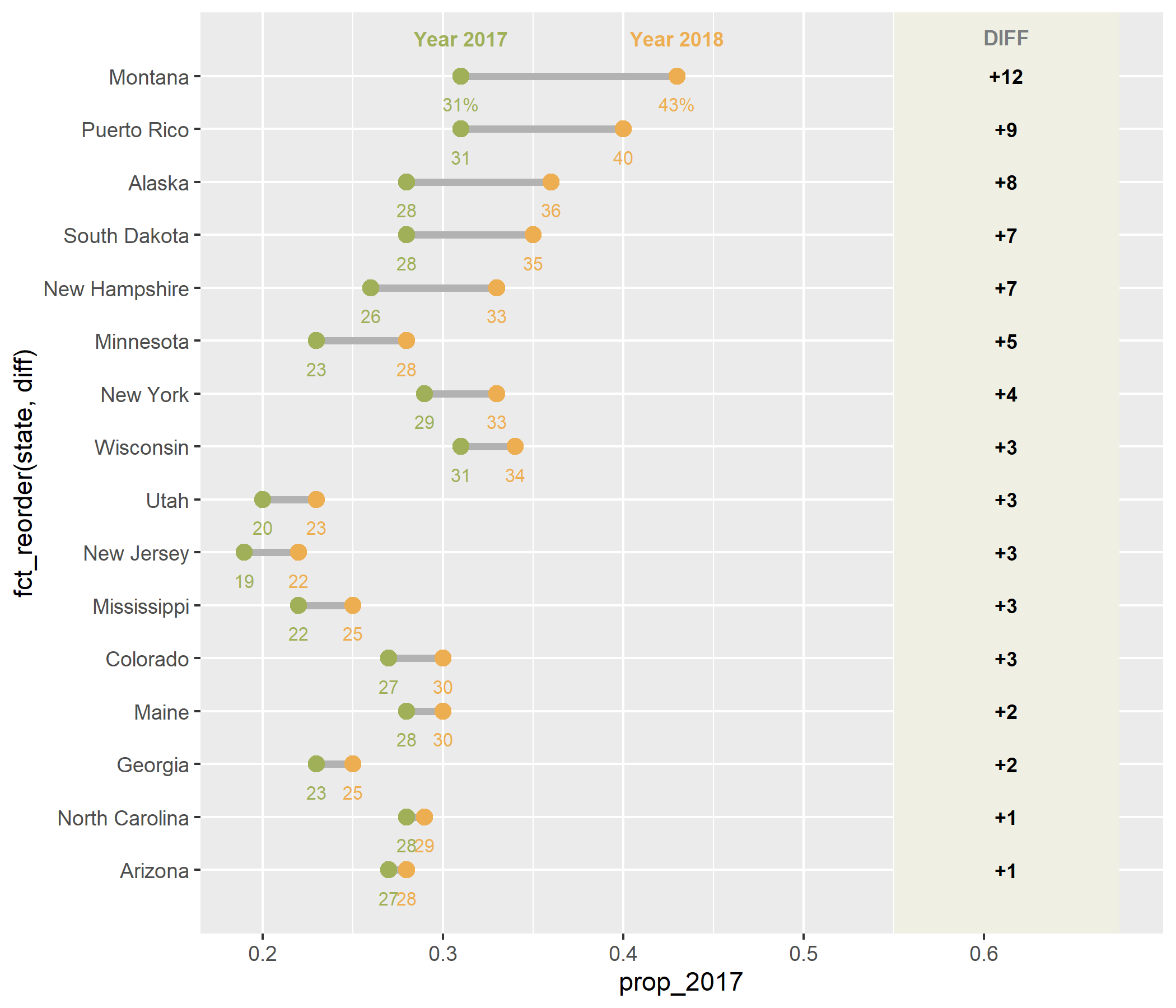
ggdumb_part3 + scale_x_continuous( expand = c(0, 0), limits = c(0, 0.675) )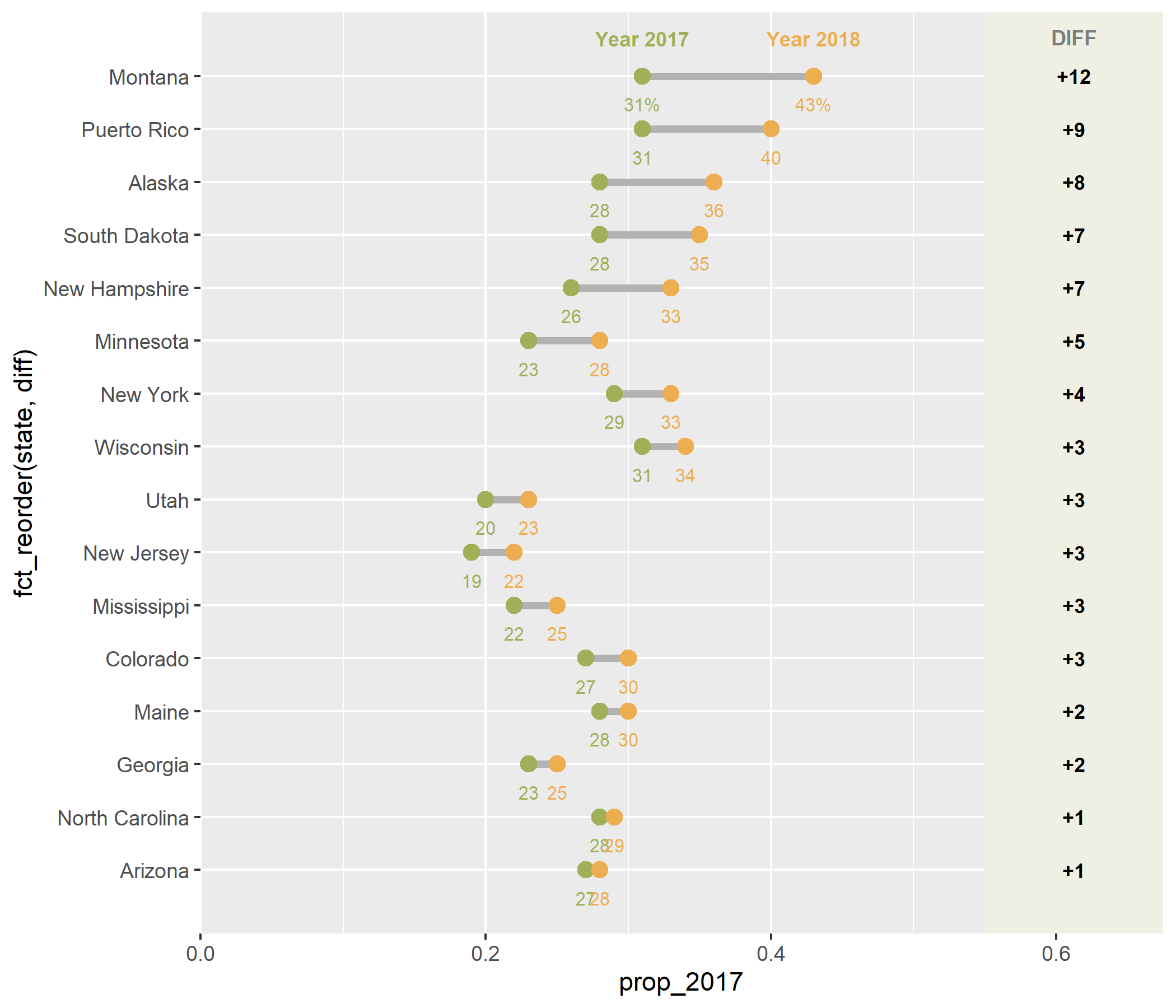
ggdumb_part3 + scale_x_continuous( expand = c(0, 0), limits = c(0, 0.675) ) + labs( x = NULL, y = NULL, title = paste( "States with alcohol problem", "based on 2017-18 comparison" ), subtitle = paste( "Alcohol-impaired-driving", "fatalities (% of total)" ), caption = "Data source: FARS" )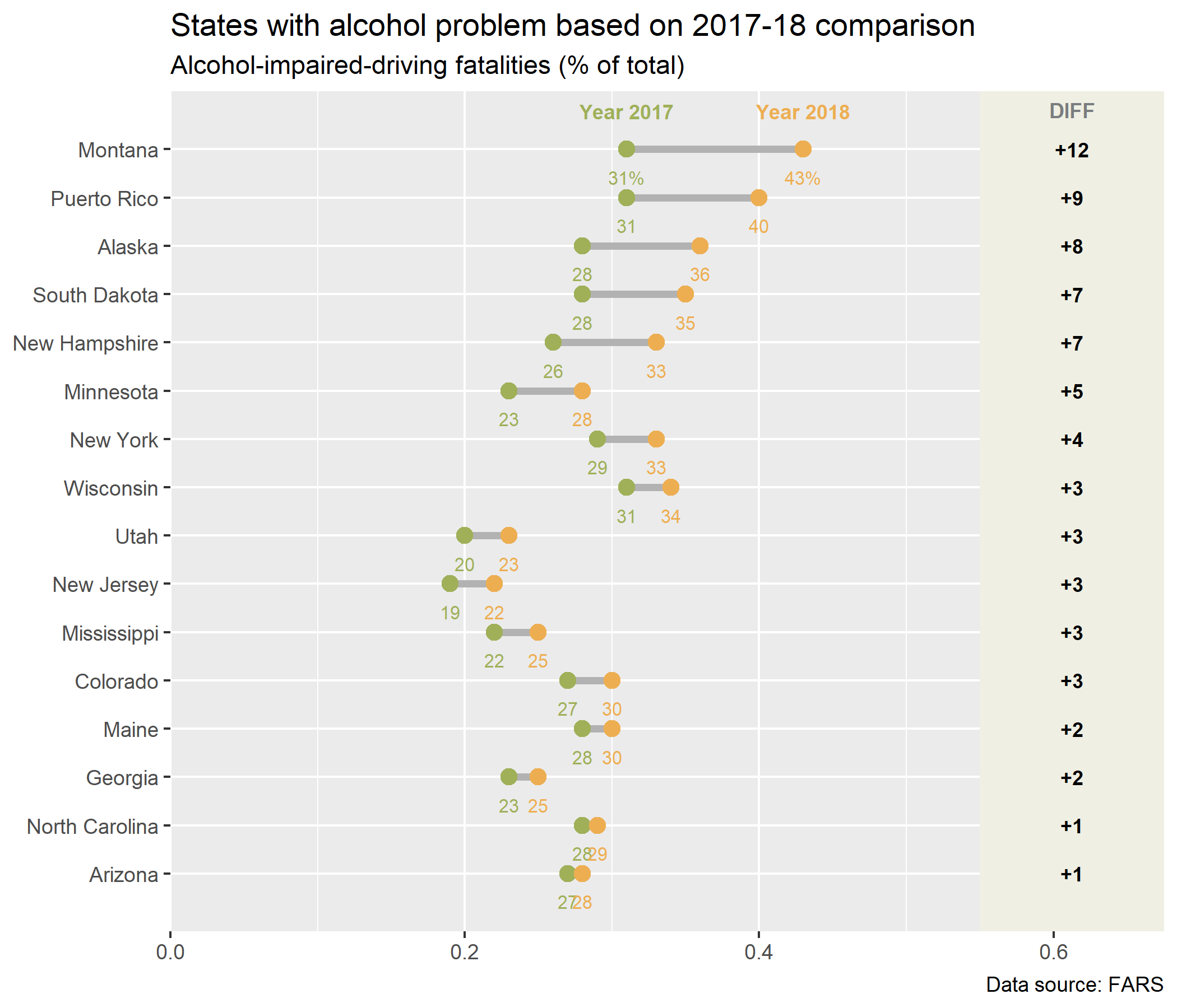
ggdumb_part3 + scale_x_continuous( expand = c(0, 0), limits = c(0, 0.675) ) + labs( x = NULL, y = NULL, title = paste( "States with alcohol problem", "based on 2017-18 comparison" ), subtitle = paste( "Alcohol-impaired-driving", "fatalities (% of total)" ), caption = "Data source: FARS" ) + theme_bw()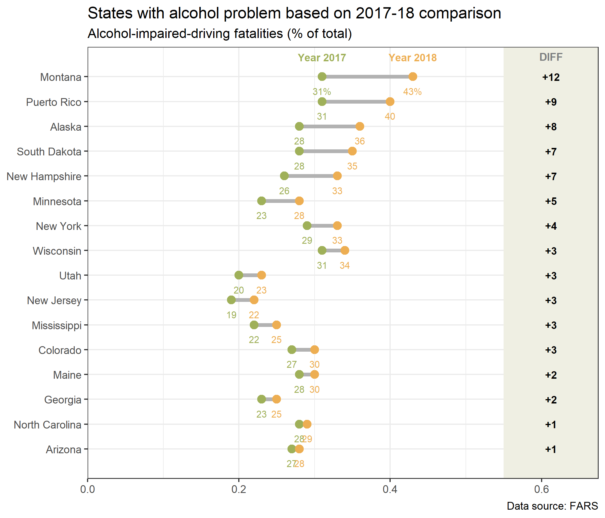
ggdumb_part3 + scale_x_continuous( expand = c(0, 0), limits = c(0, 0.675) ) + labs( x = NULL, y = NULL, title = paste( "States with alcohol problem", "based on 2017-18 comparison" ), subtitle = paste( "Alcohol-impaired-driving", "fatalities (% of total)" ), caption = "Data source: FARS" ) + theme_bw() + theme( panel.grid.major = element_blank() )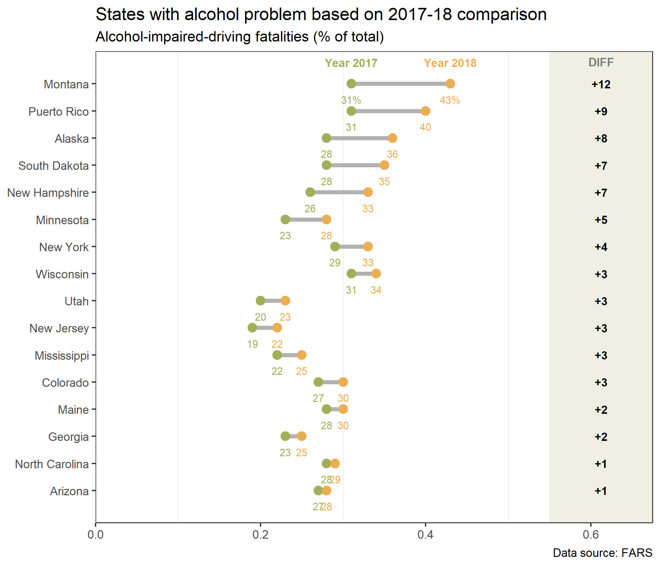
ggdumb_part3 + scale_x_continuous( expand = c(0, 0), limits = c(0, 0.675) ) + labs( x = NULL, y = NULL, title = paste( "States with alcohol problem", "based on 2017-18 comparison" ), subtitle = paste( "Alcohol-impaired-driving", "fatalities (% of total)" ), caption = "Data source: FARS" ) + theme_bw() + theme( panel.grid.major = element_blank() ) + theme( panel.grid.minor = element_blank() )
ggdumb_part3 + scale_x_continuous( expand = c(0, 0), limits = c(0, 0.675) ) + labs( x = NULL, y = NULL, title = paste( "States with alcohol problem", "based on 2017-18 comparison" ), subtitle = paste( "Alcohol-impaired-driving", "fatalities (% of total)" ), caption = "Data source: FARS" ) + theme_bw() + theme( panel.grid.major = element_blank() ) + theme( panel.grid.minor = element_blank() ) + theme( panel.border = element_blank() )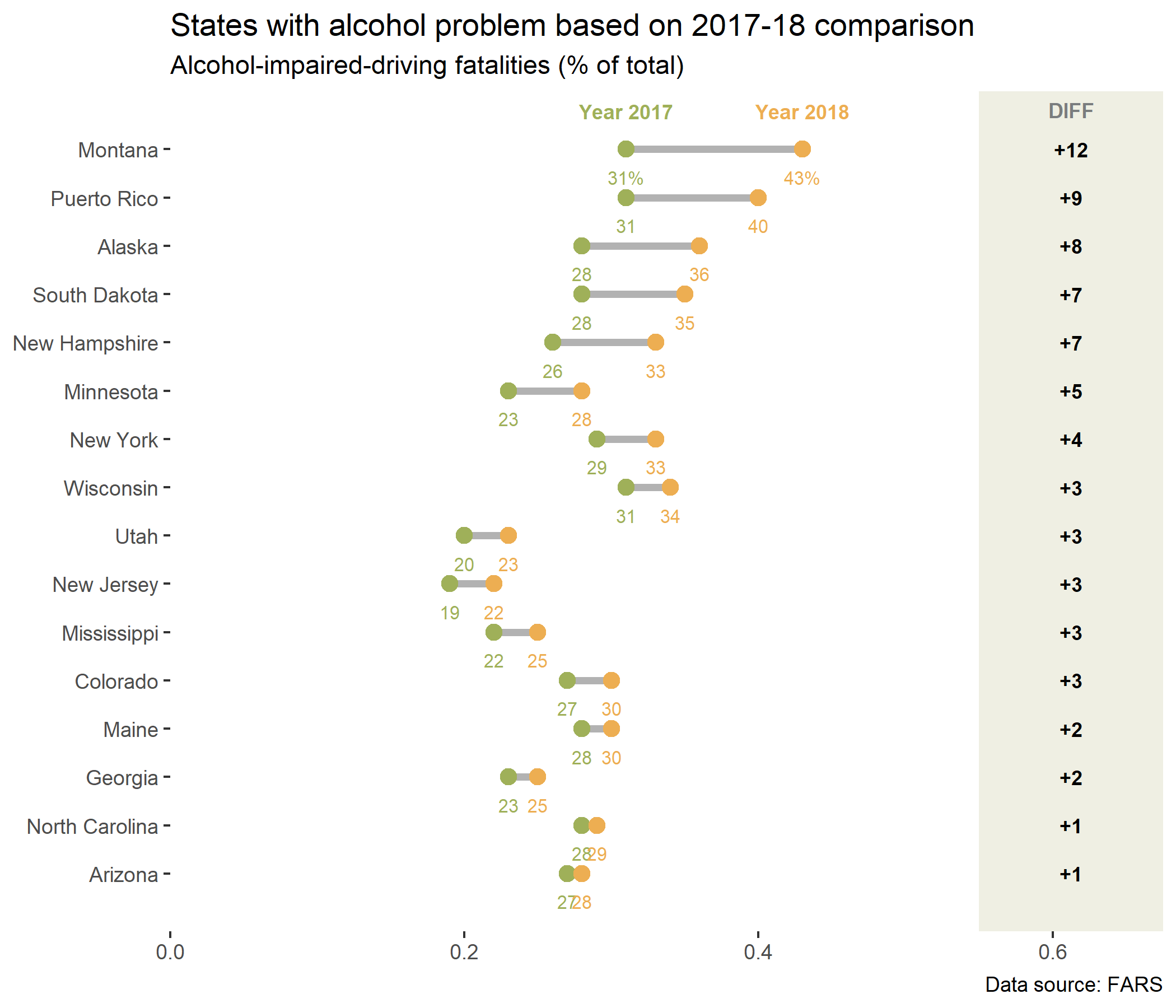
ggdumb_part4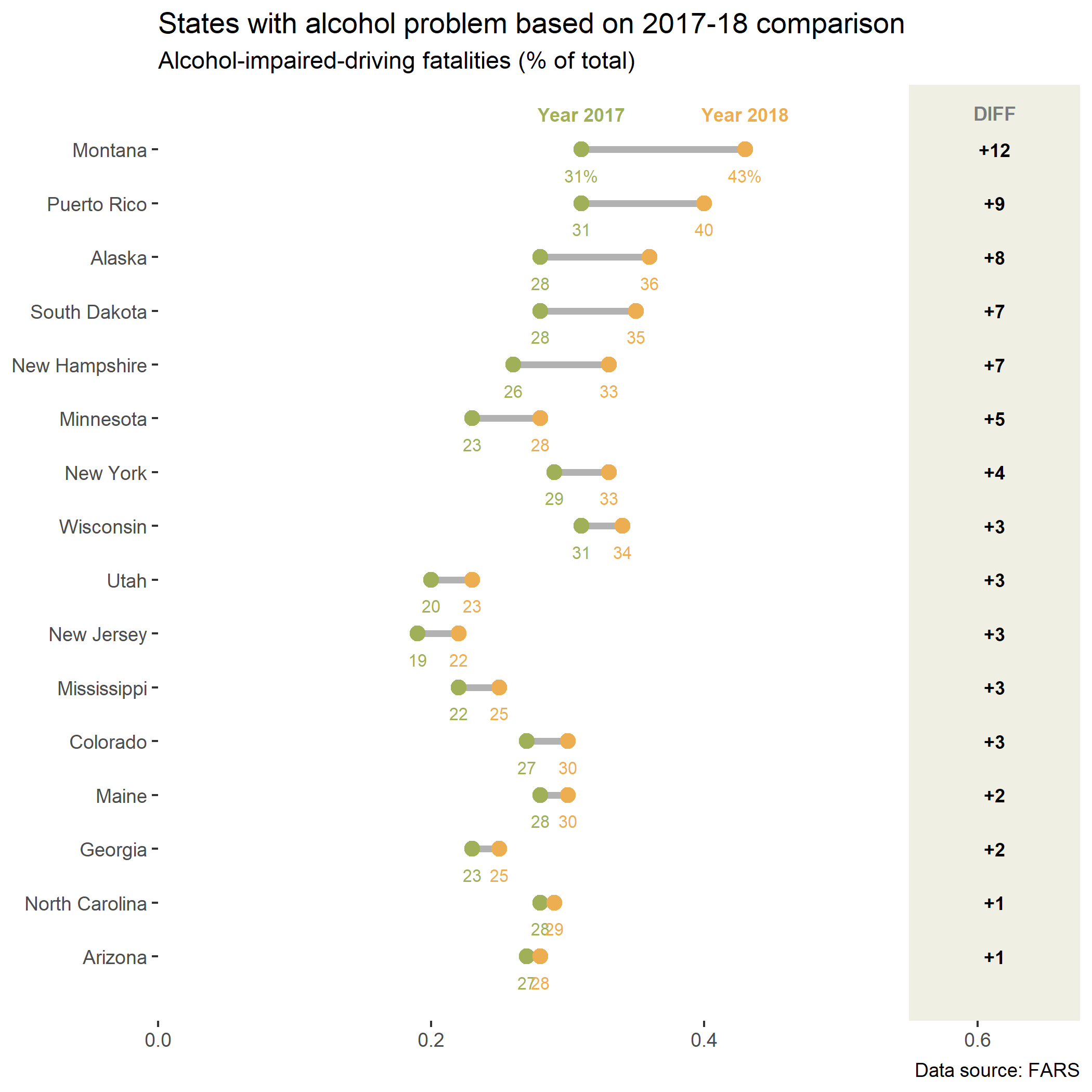
ggdumb_part4 + theme(axis.ticks = element_blank())
ggdumb_part4 + theme(axis.ticks = element_blank()) + theme(axis.text.x = element_blank())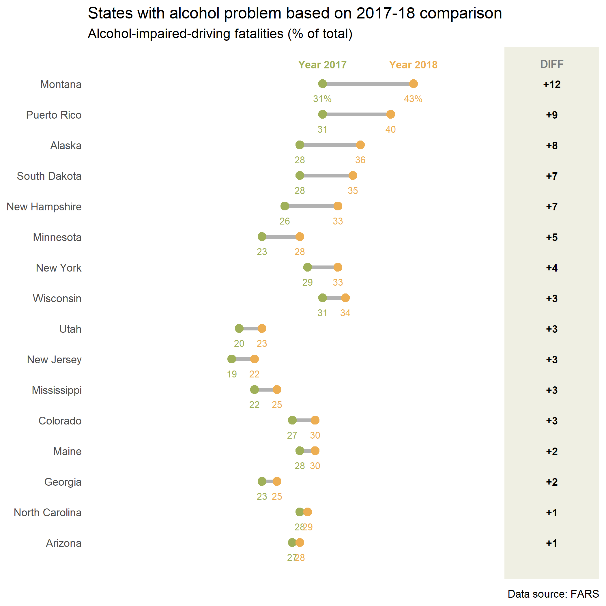
ggdumb_part4 + theme(axis.ticks = element_blank()) + theme(axis.text.x = element_blank()) + theme( plot.title = element_text( face = "bold" ) )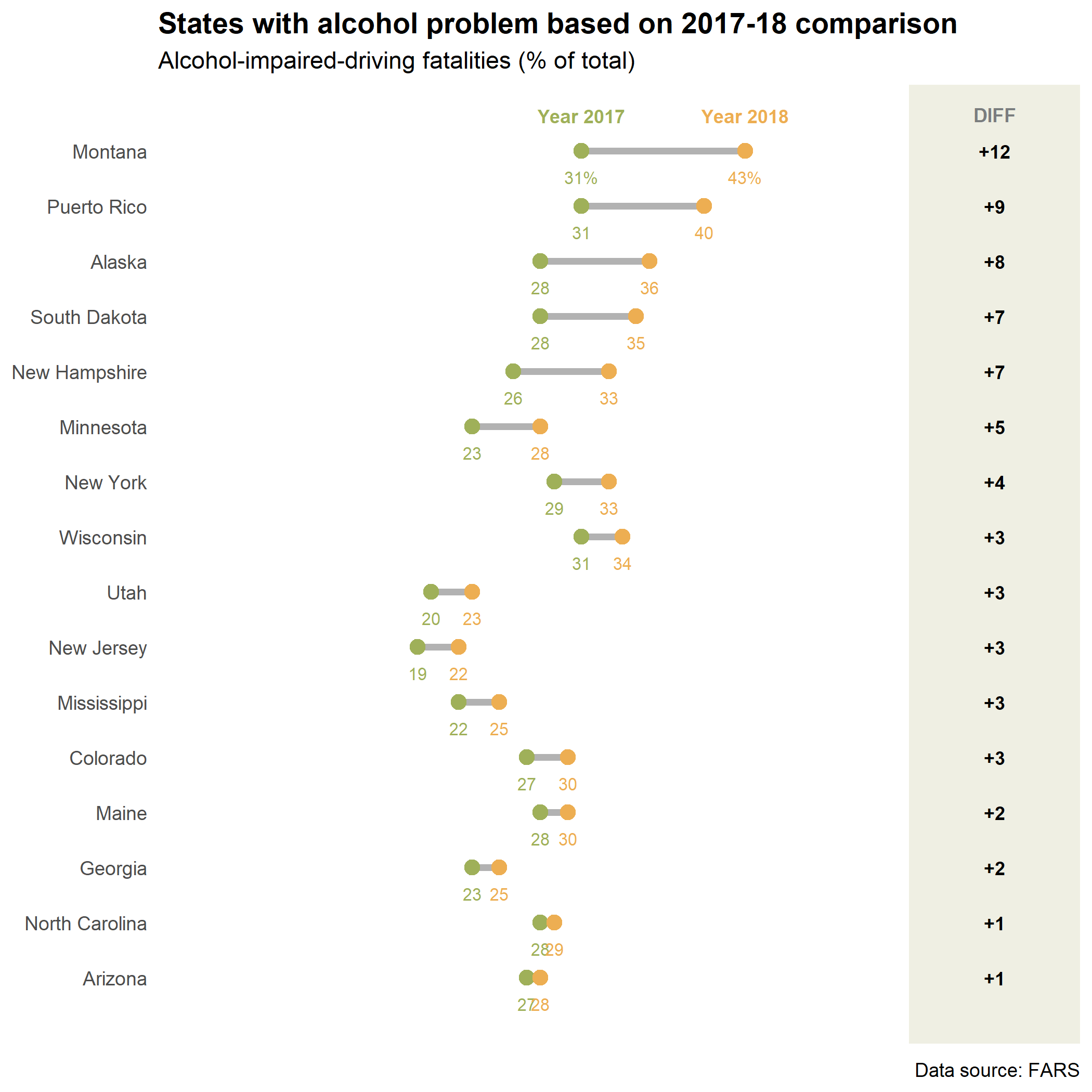
ggdumb_part4 + theme(axis.ticks = element_blank()) + theme(axis.text.x = element_blank()) + theme( plot.title = element_text( face = "bold" ) ) + theme( plot.subtitle = element_text( face = "italic", size = 9, margin = margin(b = 12) ) )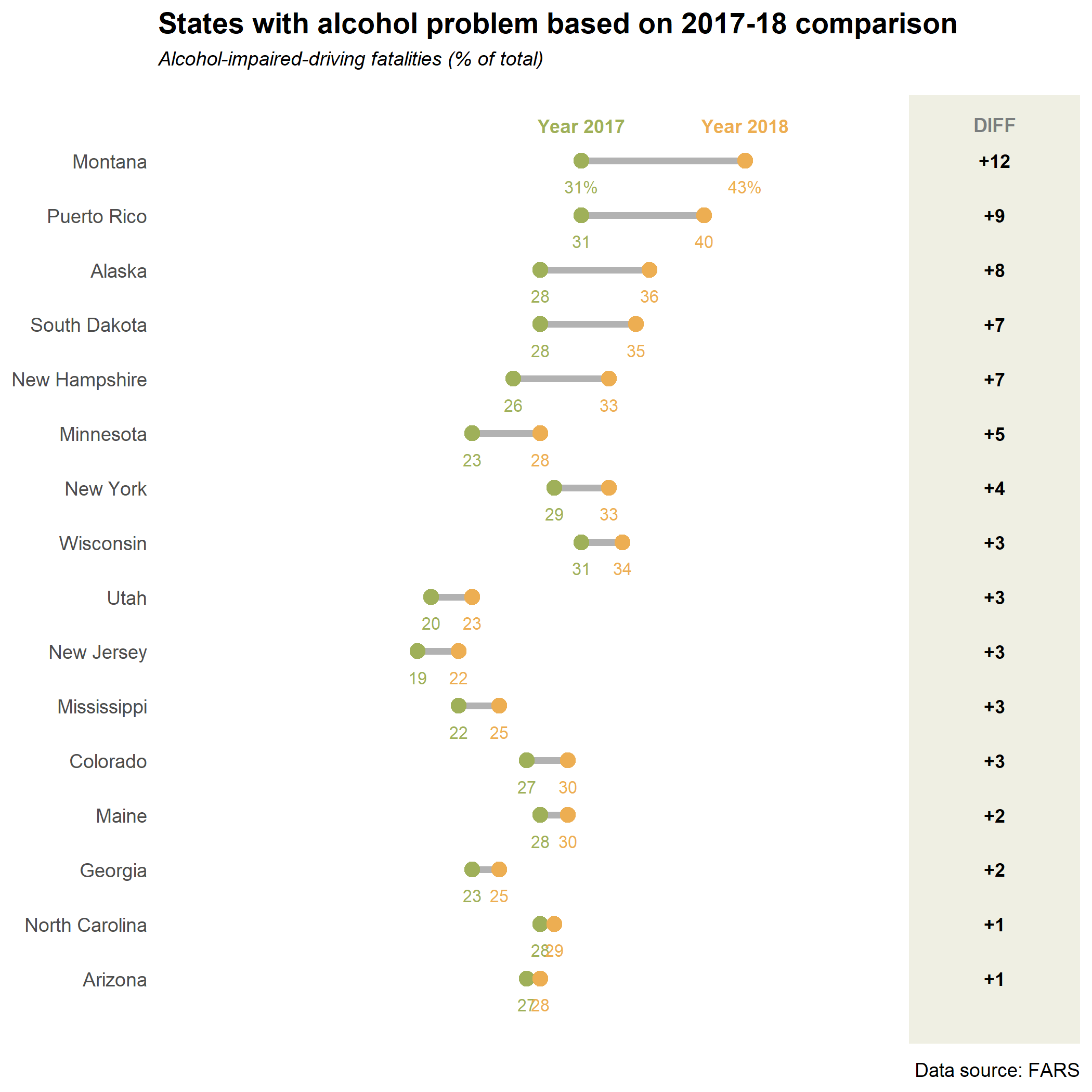
ggdumb_part4 + theme(axis.ticks = element_blank()) + theme(axis.text.x = element_blank()) + theme( plot.title = element_text( face = "bold" ) ) + theme( plot.subtitle = element_text( face = "italic", size = 9, margin = margin(b = 12) ) ) + theme( plot.caption = element_text( size = 7, margin = margin(t = 12), color = "#7a7d7e" ) )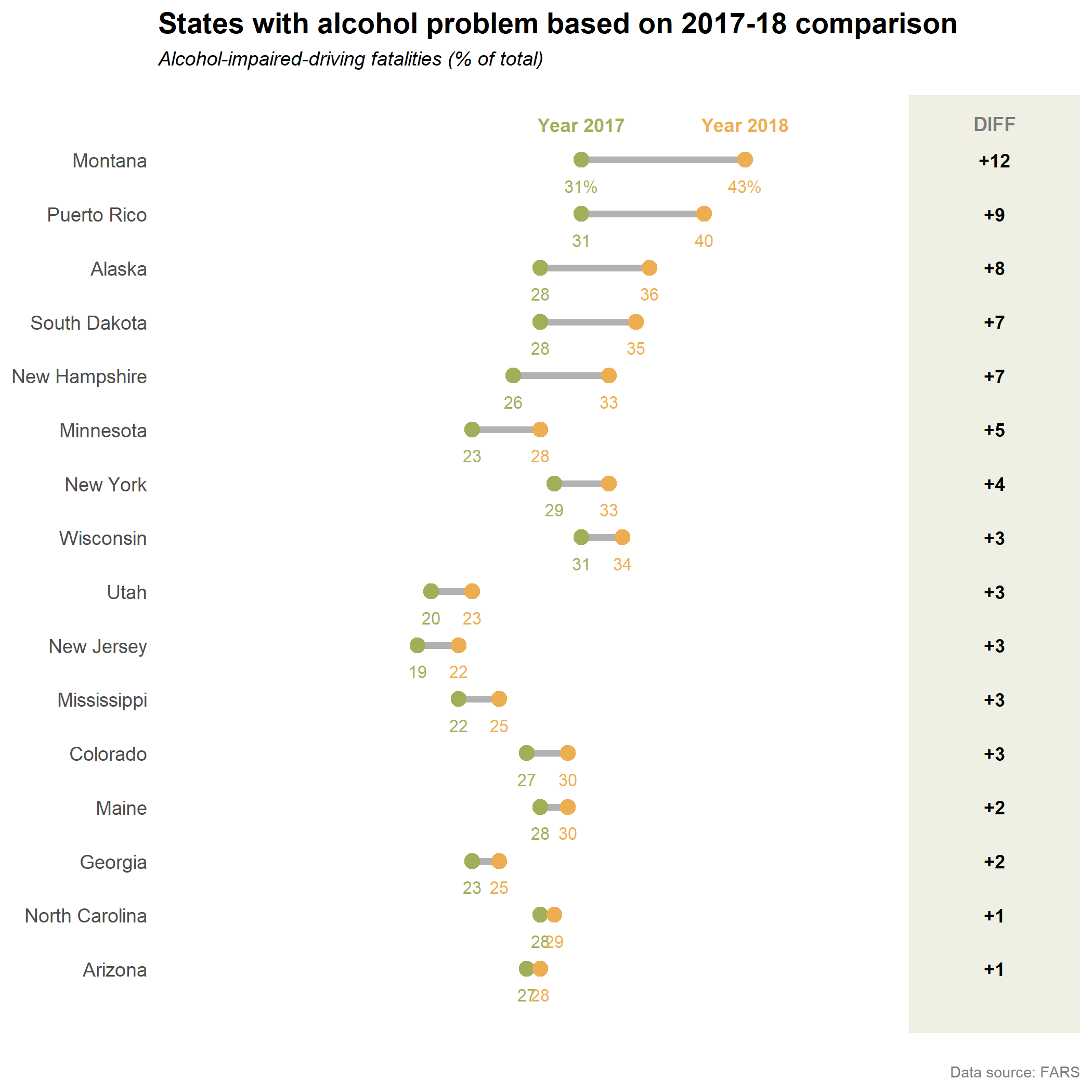
ggdumb_part4 + theme(axis.ticks = element_blank()) + theme(axis.text.x = element_blank()) + theme( plot.title = element_text( face = "bold" ) ) + theme( plot.subtitle = element_text( face = "italic", size = 9, margin = margin(b = 12) ) ) + theme( plot.caption = element_text( size = 7, margin = margin(t = 12), color = "#7a7d7e" ) ) + geom_segment( aes( y = state, yend = state, x = 0, xend = 0.5 ), color = "#b2b2b2", size = 0.15 )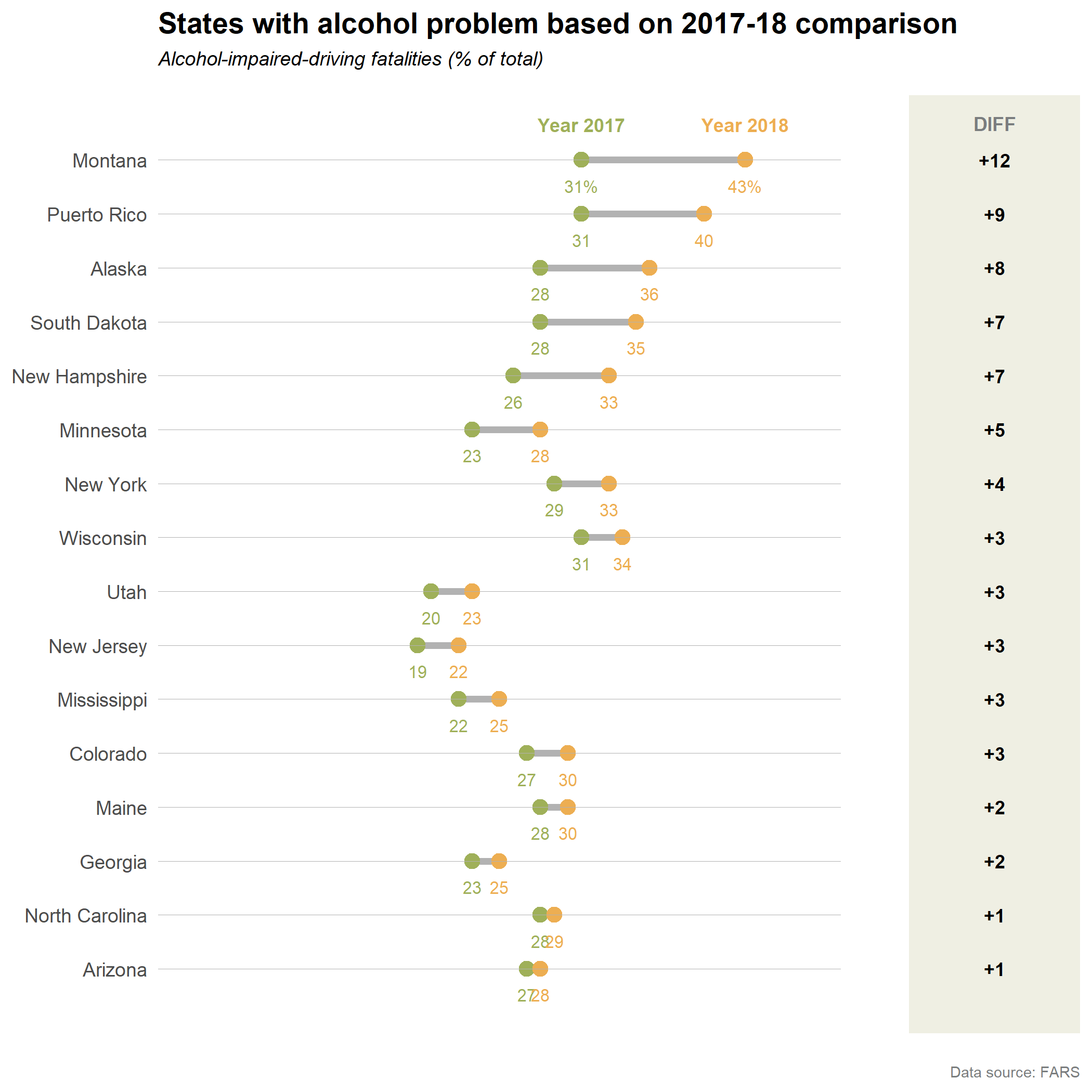
fatal_crash_smry_by_state %>% slice_max(death_rate_vmt, n = 2) -> ggspike_dffatal_crash_smry_by_state %>% ggplot( aes( x = death_rate_vmt, y = death_rate_pop ) )
fatal_crash_smry_by_state %>% slice_max(death_rate_vmt, n = 2) -> ggspike_dffatal_crash_smry_by_state %>% ggplot( aes( x = death_rate_vmt, y = death_rate_pop ) ) + geom_point()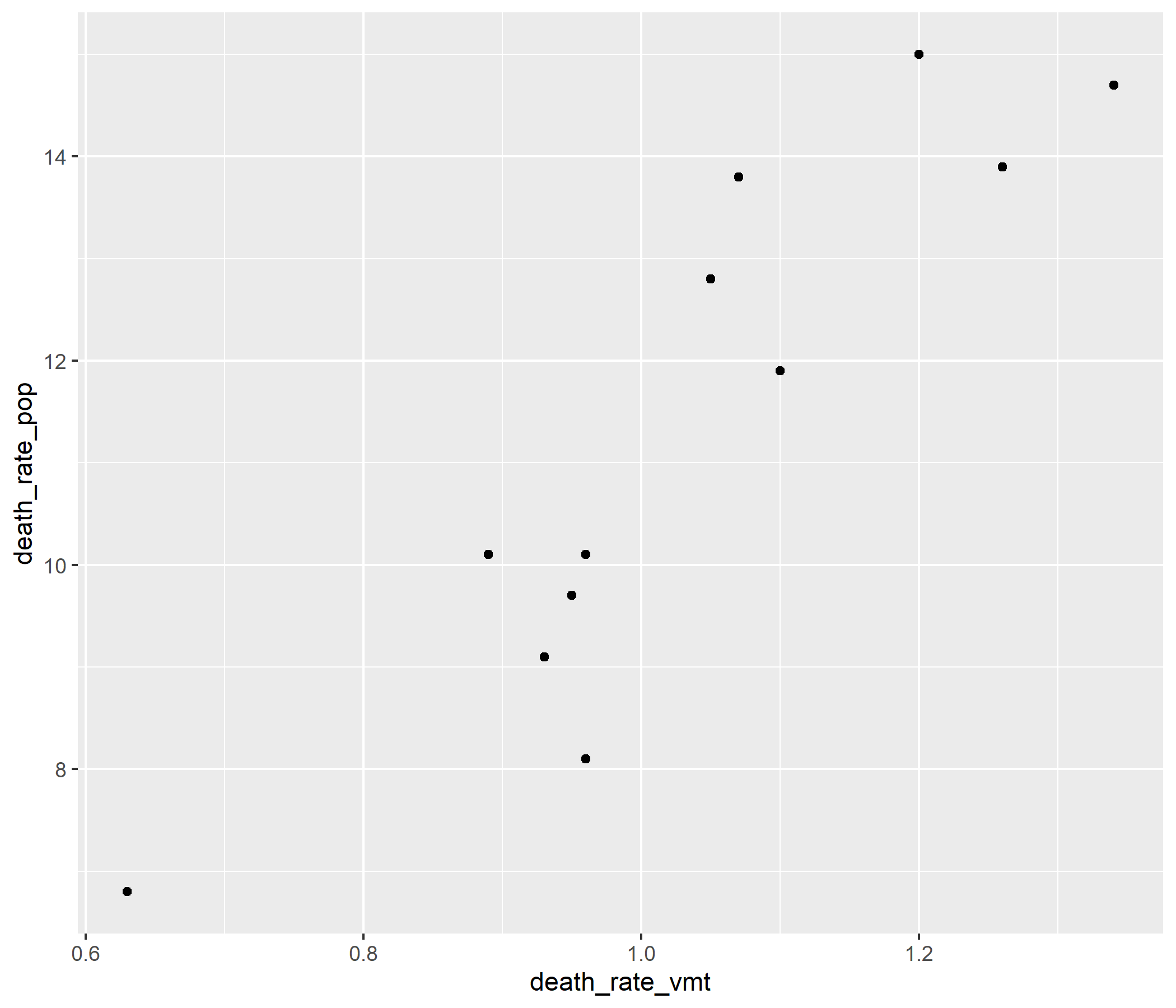
fatal_crash_smry_by_state %>% slice_max(death_rate_vmt, n = 2) -> ggspike_dffatal_crash_smry_by_state %>% ggplot( aes( x = death_rate_vmt, y = death_rate_pop ) ) + geom_point() + geom_encircle( data = ggspike_df, color = "red", s_shape = 0.3, expand = 0.03, spread = 0.01 )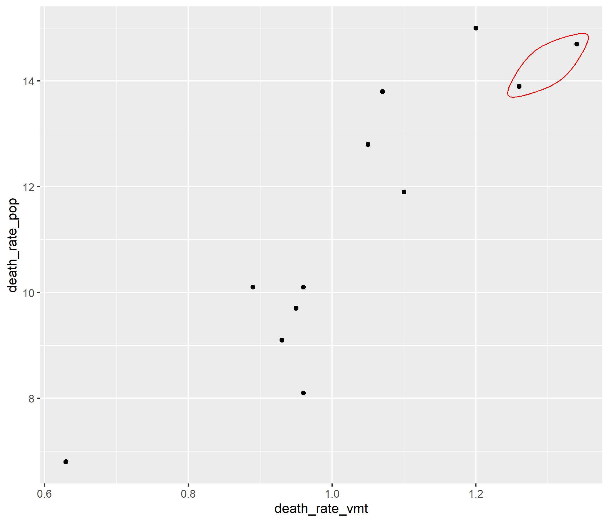
fatal_crash_smry_by_state %>% slice_max(death_rate_vmt, n = 2) -> ggspike_dffatal_crash_smry_by_state %>% ggplot( aes( x = death_rate_vmt, y = death_rate_pop ) ) + geom_point() + geom_encircle( data = ggspike_df, color = "red", s_shape = 0.3, expand = 0.03, spread = 0.01 ) + geom_point( data = ggspike_df, color = "red" )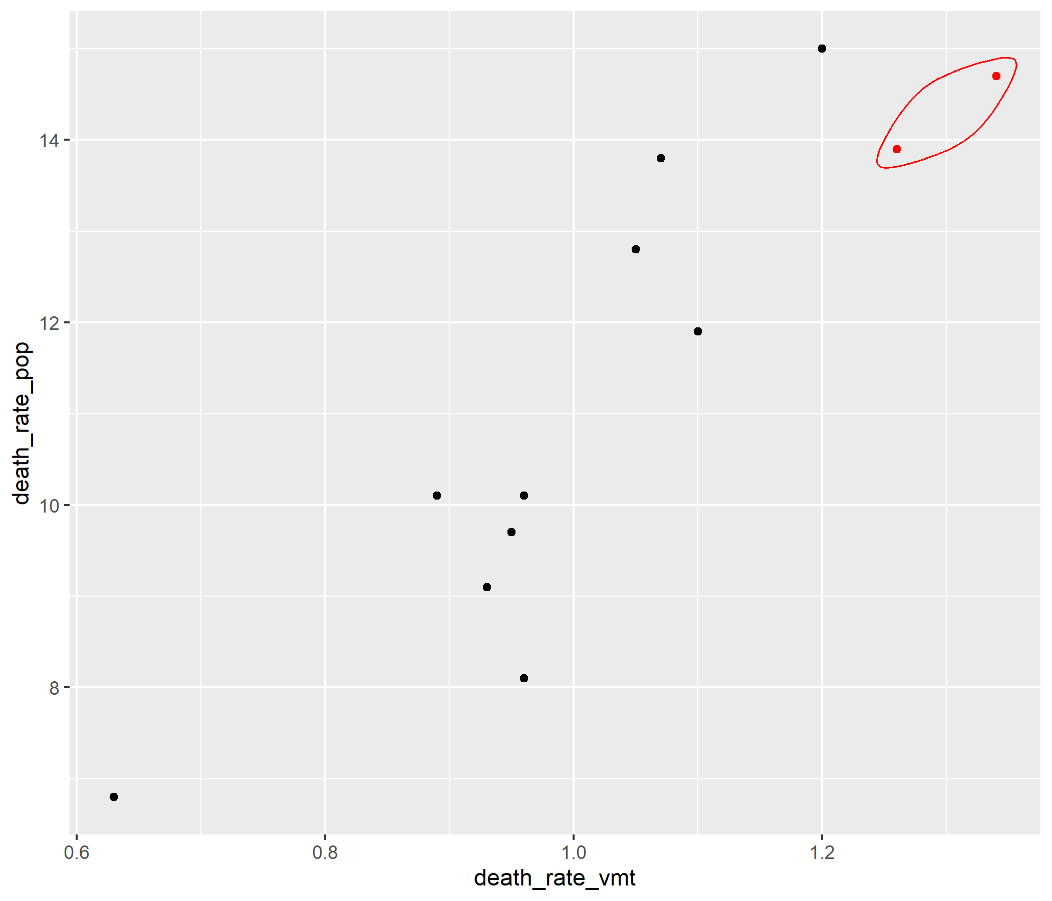
fatal_crash_smry_by_state %>% slice_max(death_rate_vmt, n = 2) -> ggspike_dffatal_crash_smry_by_state %>% ggplot( aes( x = death_rate_vmt, y = death_rate_pop ) ) + geom_point() + geom_encircle( data = ggspike_df, color = "red", s_shape = 0.3, expand = 0.03, spread = 0.01 ) + geom_point( data = ggspike_df, color = "red" ) + geom_spikelines( data = ggspike_df, linetype = 2 )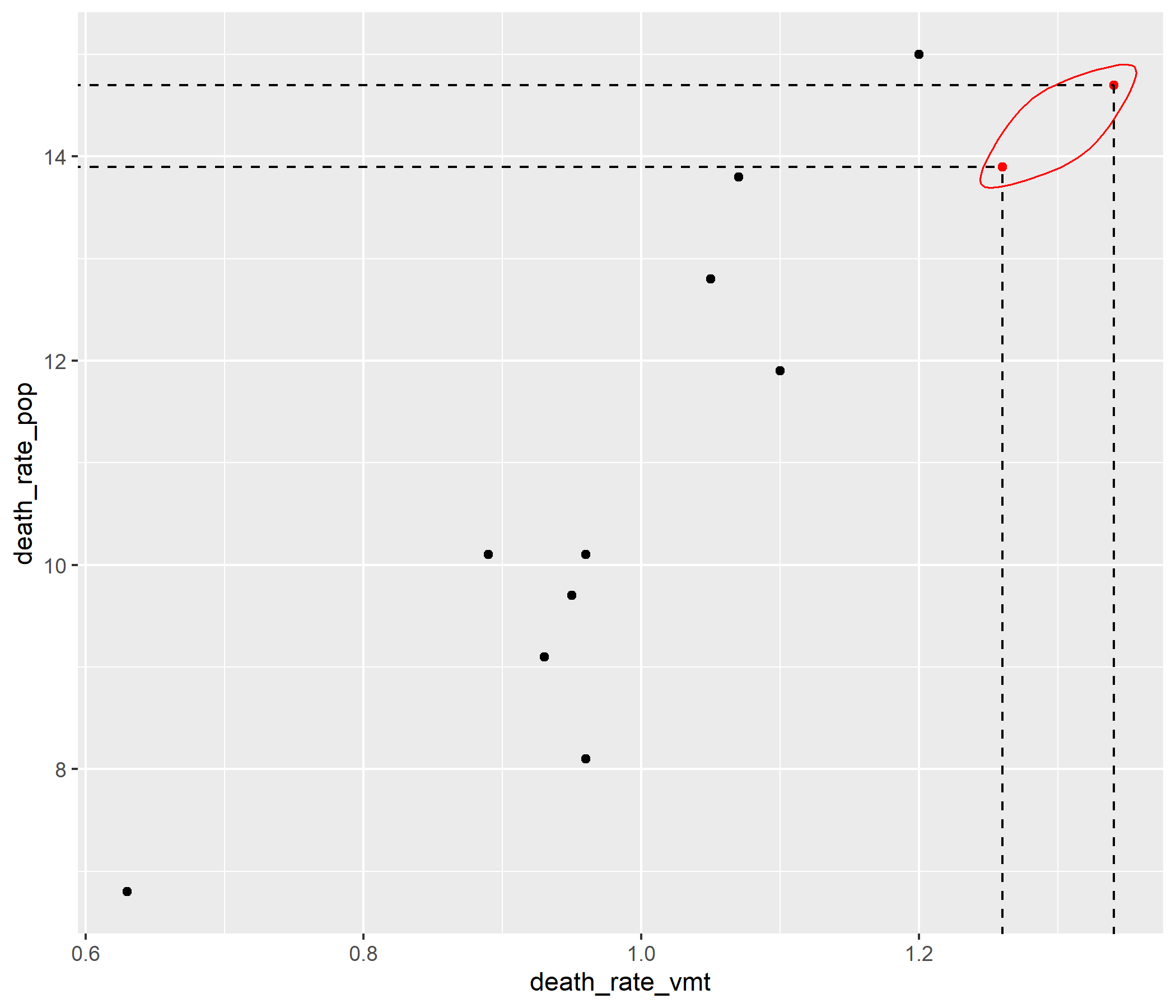
ggspike_part1
ggspike_part1 + geom_label_repel( data = ggspike_df, aes( label = glue( "({death_rate_vmt}, ", "{death_rate_pop})" ) ), box.padding = 1, color = "red" )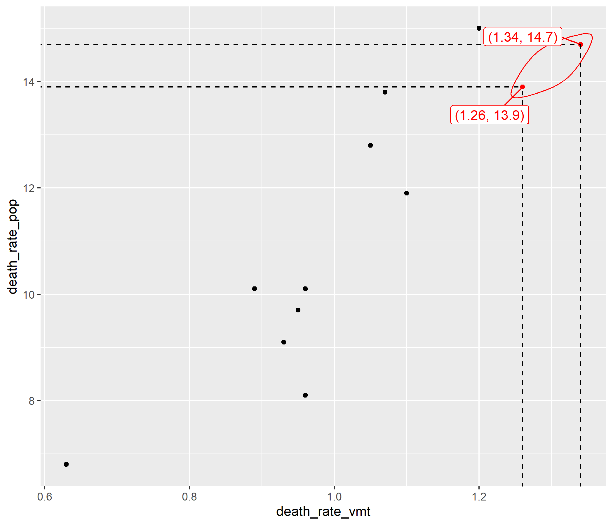
ggspike_part1 + geom_label_repel( data = ggspike_df, aes( label = glue( "({death_rate_vmt}, ", "{death_rate_pop})" ) ), box.padding = 1, color = "red" ) + labs( x = "Deaths per 100 million VMT", y = "Deaths per 100k population", title = paste( "Relationship between motor", "vehicle crash death rates", "for midwest, 2018" ), caption = "Data source: IIHS" )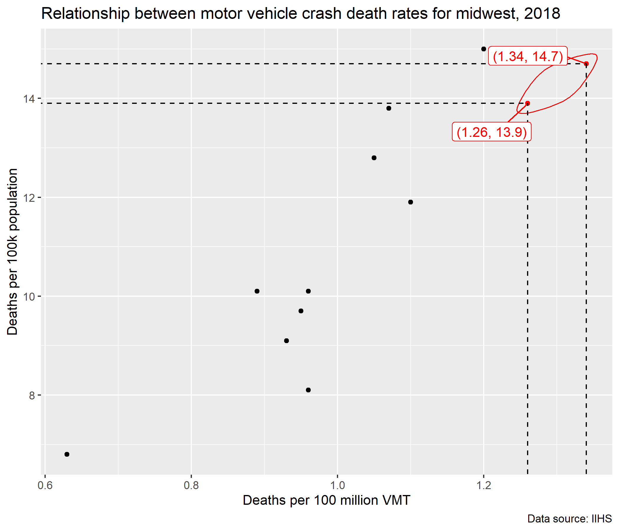
fatal_crash_monthly_counts %>% ggplot( aes( x = fatal_crash_freq, y = crash_month, fill = stat(x) ) )
fatal_crash_monthly_counts %>% ggplot( aes( x = fatal_crash_freq, y = crash_month, fill = stat(x) ) ) + geom_density_ridges_gradient( scale = 3, rel_min_height = 0.01 )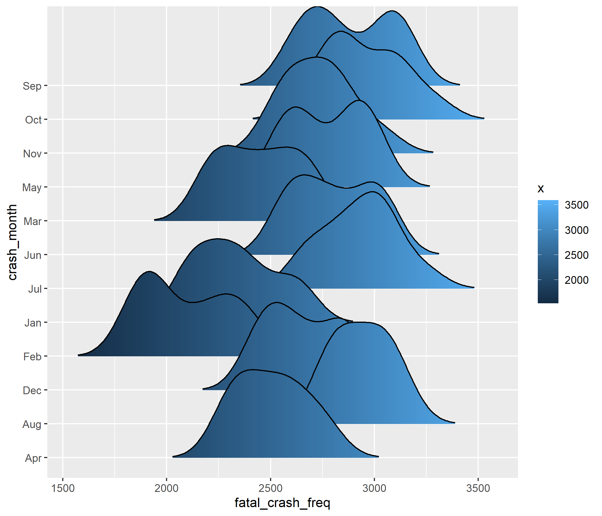
fatal_crash_monthly_counts %>% ggplot( aes( x = fatal_crash_freq, y = crash_month, fill = stat(x) ) ) + geom_density_ridges_gradient( scale = 3, rel_min_height = 0.01 ) + scale_y_discrete( limits = rev(month.abb) )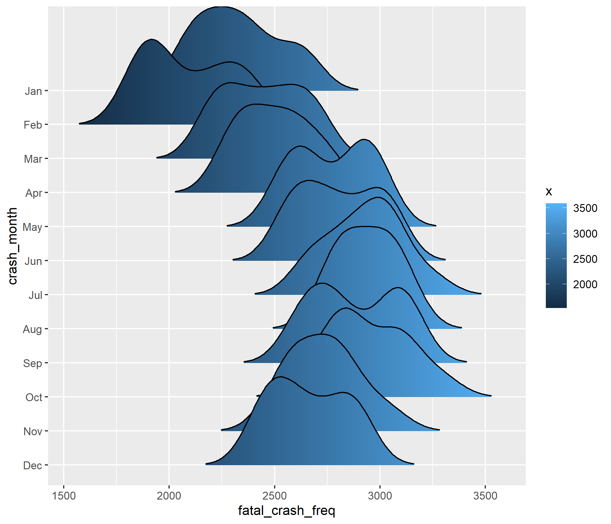
fatal_crash_monthly_counts %>% ggplot( aes( x = fatal_crash_freq, y = crash_month, fill = stat(x) ) ) + geom_density_ridges_gradient( scale = 3, rel_min_height = 0.01 ) + scale_y_discrete( limits = rev(month.abb) ) + scale_fill_viridis_c( name = "Fatal Crash Freq.", option = "C" )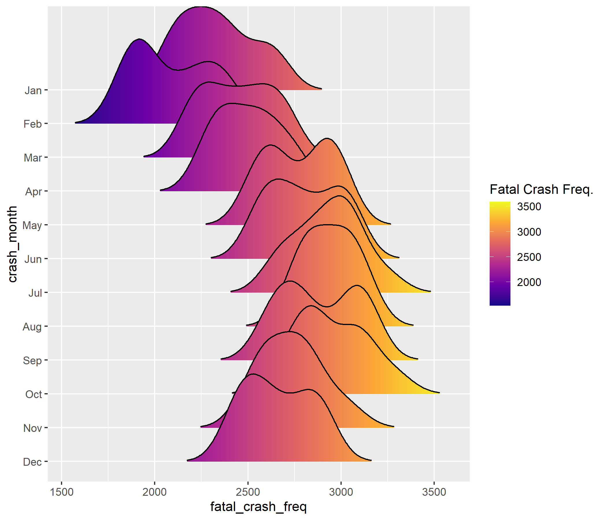
fatal_crash_monthly_counts %>% ggplot( aes( x = fatal_crash_freq, y = crash_month, fill = stat(x) ) ) + geom_density_ridges_gradient( scale = 3, rel_min_height = 0.01 ) + scale_y_discrete( limits = rev(month.abb) ) + scale_fill_viridis_c( name = "Fatal Crash Freq.", option = "C" ) + labs( x = "Fatal crash frequency", y = "Crash month", title = paste( "Motor vehicle monthly fatal", "crashes in the U.S., 2010–2019" ) )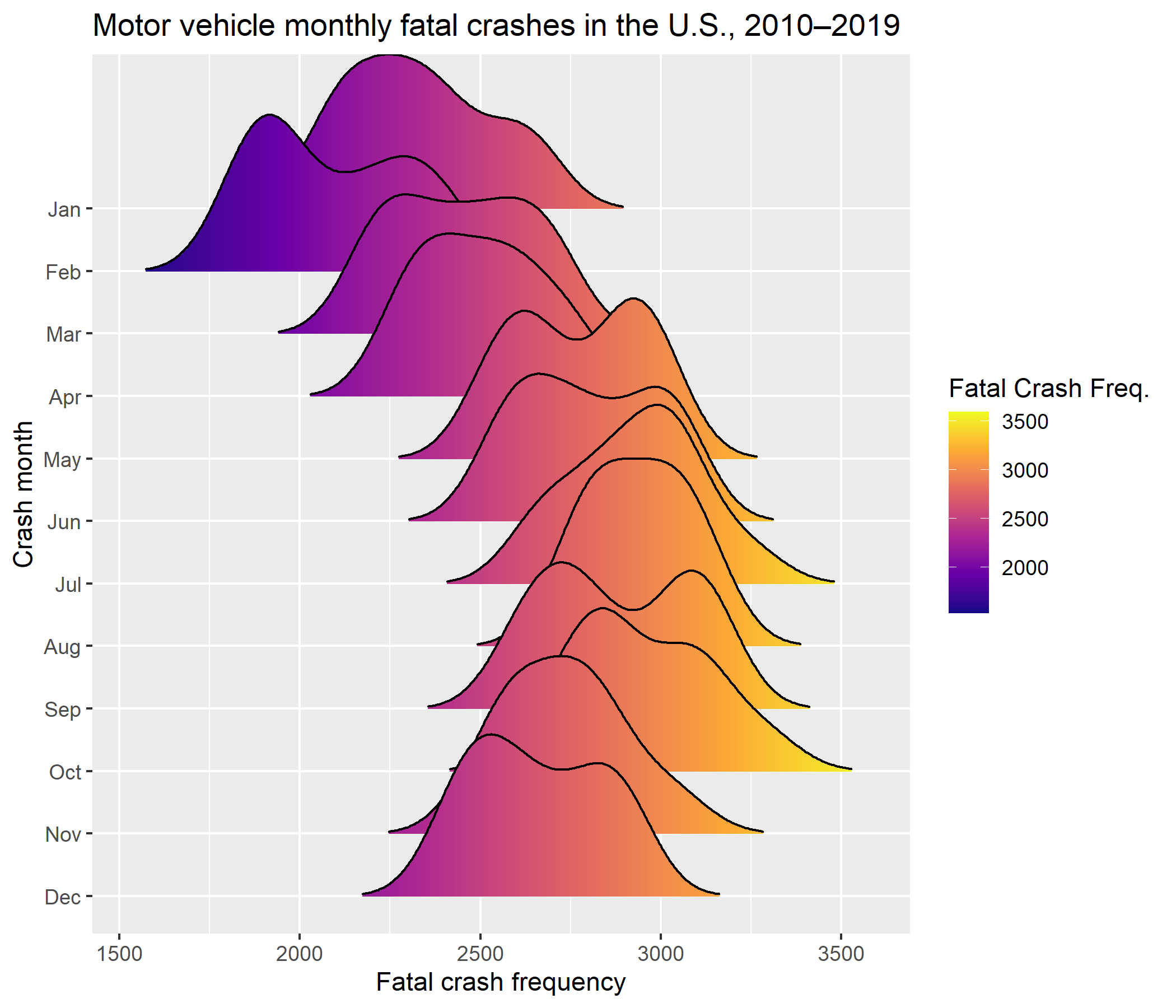
ggplot( ggimage_df, aes( x = fct_reorder( country, deaths_per_100k_pop ), y = deaths_per_100k_pop ))
ggplot( ggimage_df, aes( x = fct_reorder( country, deaths_per_100k_pop ), y = deaths_per_100k_pop )) + geom_point()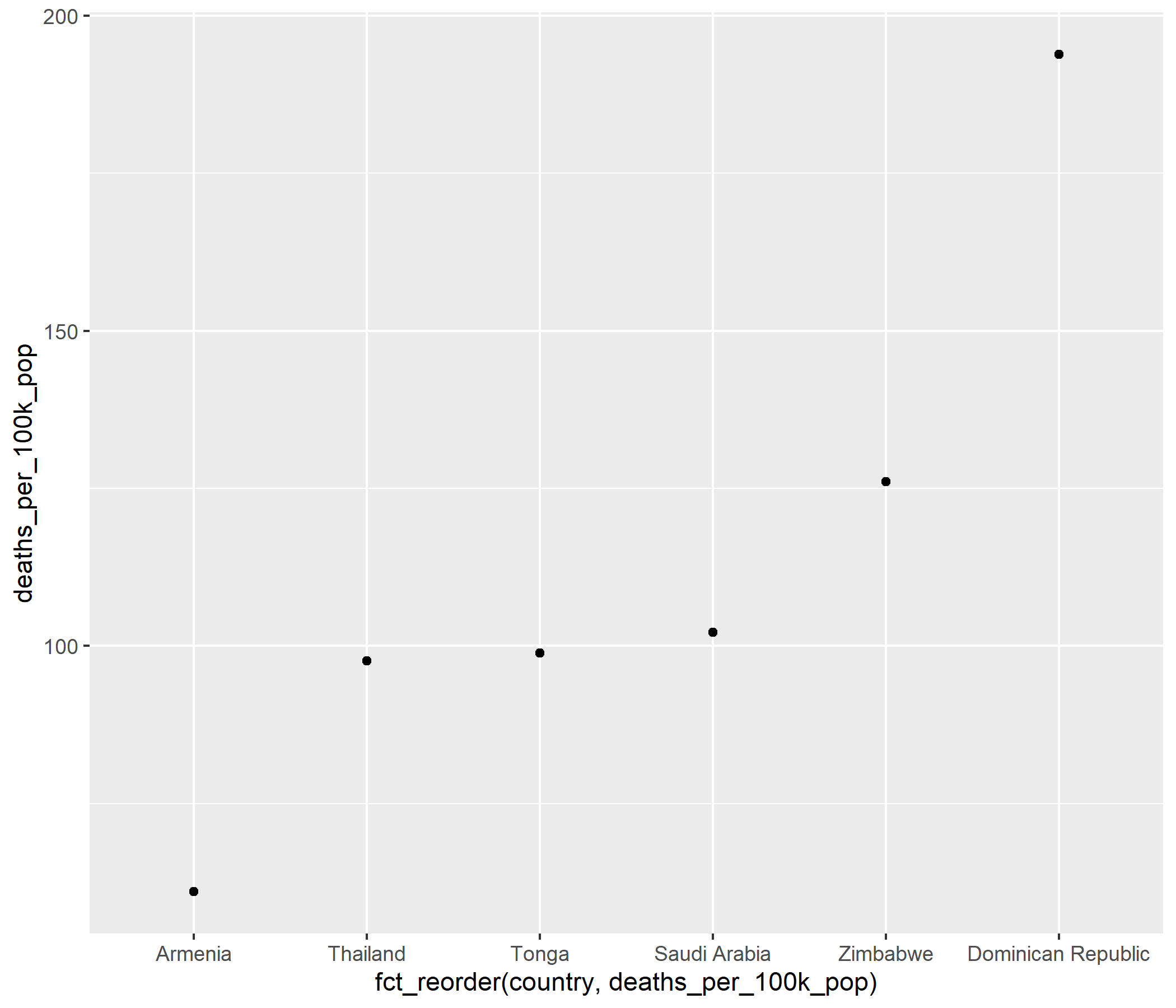
ggplot( ggimage_df, aes( x = fct_reorder( country, deaths_per_100k_pop ), y = deaths_per_100k_pop )) + geom_point() + geom_segment( aes( y = 0, yend = deaths_per_100k_pop, x = country, xend = country ) )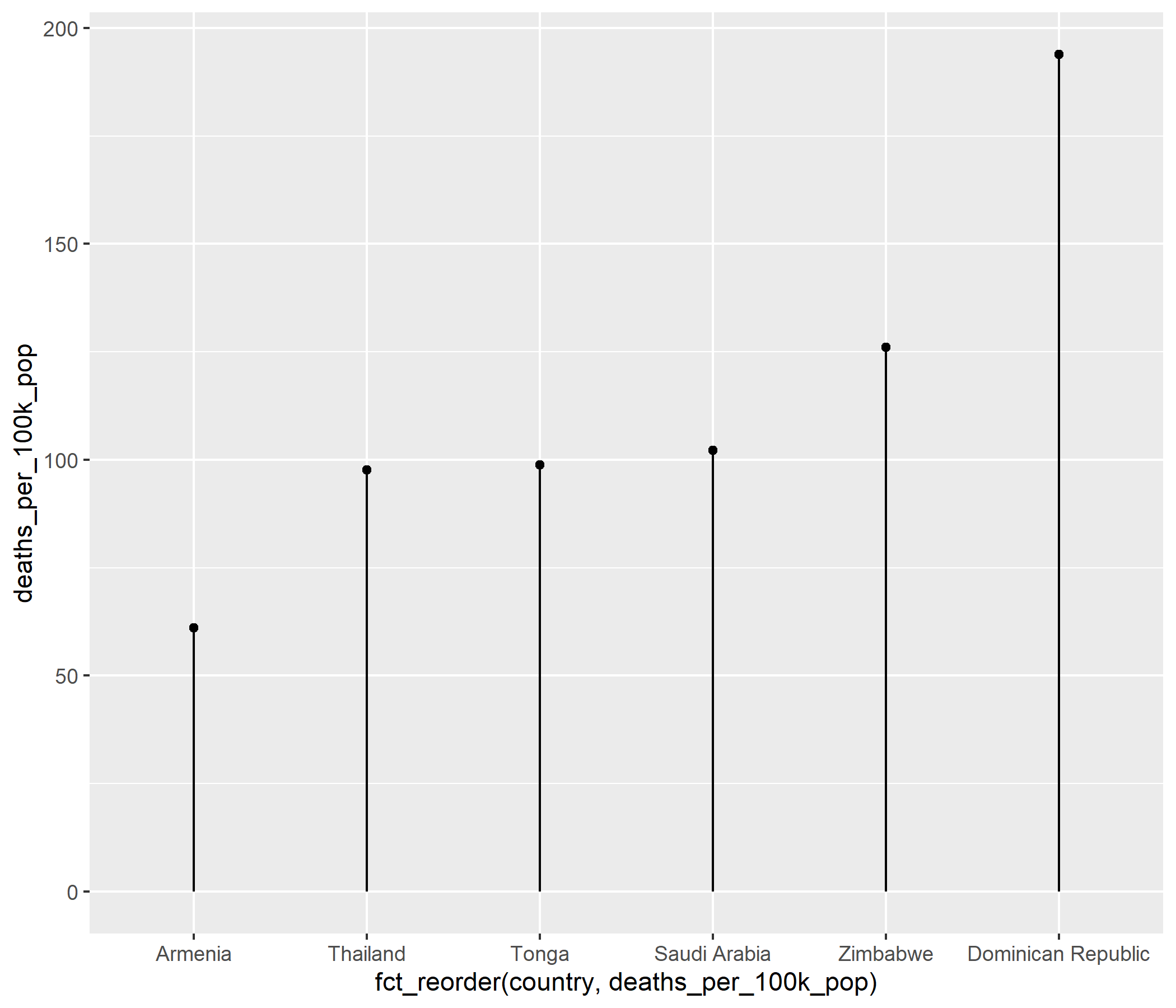
ggplot( ggimage_df, aes( x = fct_reorder( country, deaths_per_100k_pop ), y = deaths_per_100k_pop )) + geom_point() + geom_segment( aes( y = 0, yend = deaths_per_100k_pop, x = country, xend = country ) ) + geom_flag( y = -8, aes(image = country_code) )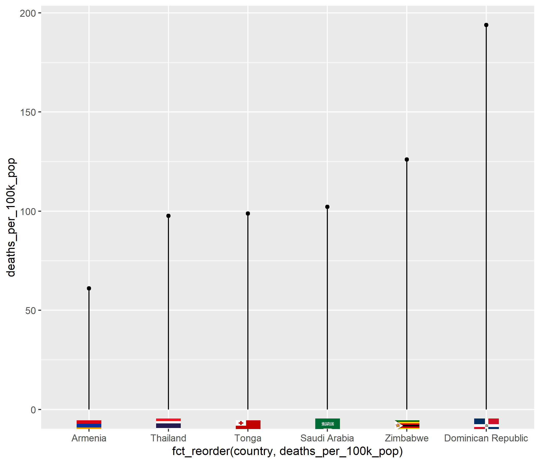
ggplot( ggimage_df, aes( x = fct_reorder( country, deaths_per_100k_pop ), y = deaths_per_100k_pop )) + geom_point() + geom_segment( aes( y = 0, yend = deaths_per_100k_pop, x = country, xend = country ) ) + geom_flag( y = -8, aes(image = country_code) ) + coord_flip()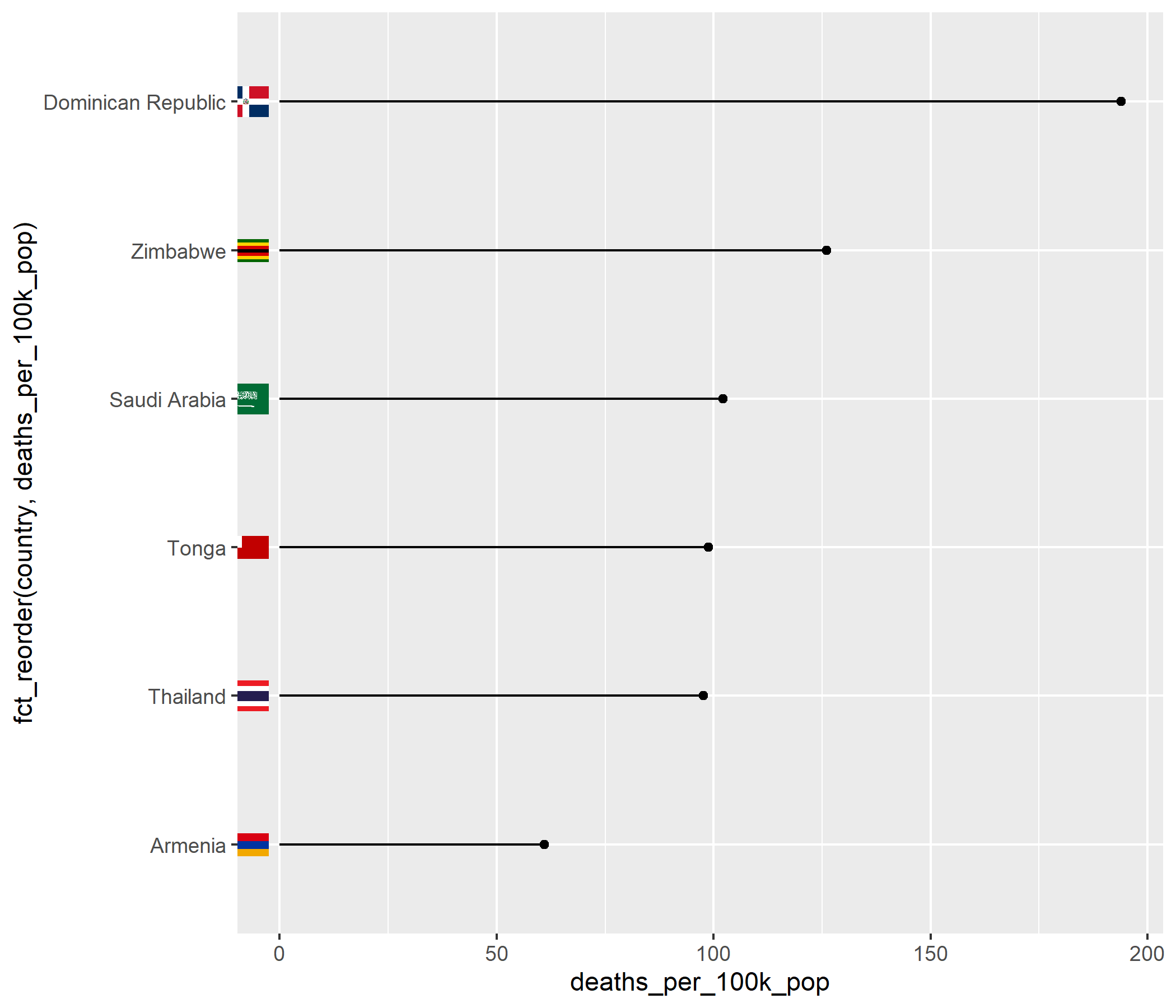
ggplot( ggimage_df, aes( x = fct_reorder( country, deaths_per_100k_pop ), y = deaths_per_100k_pop )) + geom_point() + geom_segment( aes( y = 0, yend = deaths_per_100k_pop, x = country, xend = country ) ) + geom_flag( y = -8, aes(image = country_code) ) + coord_flip() + expand_limits(y = -8)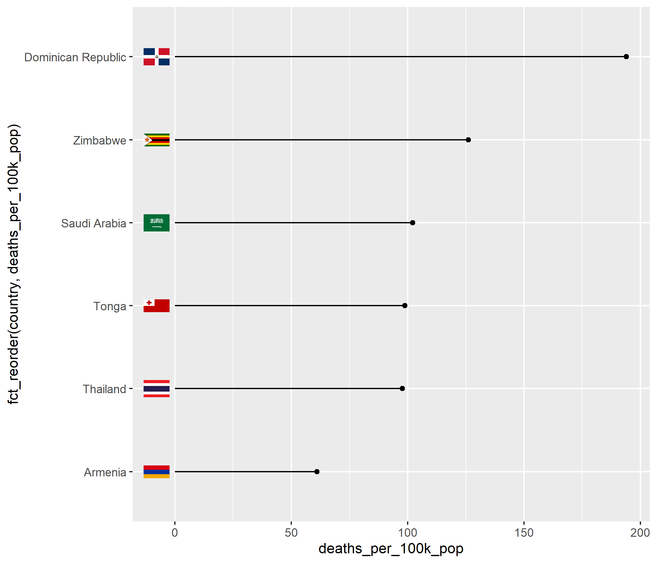
ggplot( ggimage_df, aes( x = fct_reorder( country, deaths_per_100k_pop ), y = deaths_per_100k_pop )) + geom_point() + geom_segment( aes( y = 0, yend = deaths_per_100k_pop, x = country, xend = country ) ) + geom_flag( y = -8, aes(image = country_code) ) + coord_flip() + expand_limits(y = -8) + theme_minimal()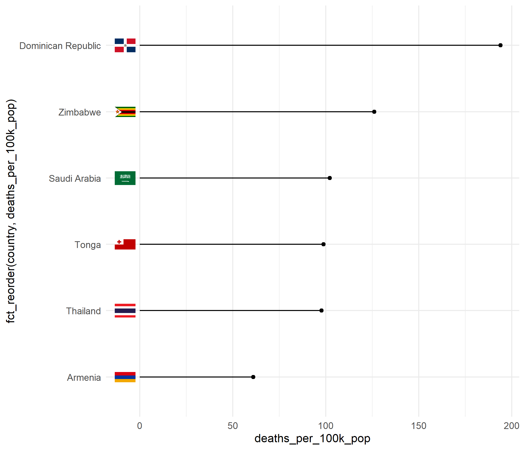
ggplot( ggimage_df, aes( x = fct_reorder( country, deaths_per_100k_pop ), y = deaths_per_100k_pop )) + geom_point() + geom_segment( aes( y = 0, yend = deaths_per_100k_pop, x = country, xend = country ) ) + geom_flag( y = -8, aes(image = country_code) ) + coord_flip() + expand_limits(y = -8) + theme_minimal() + theme(axis.title = element_blank())
ggimage_part1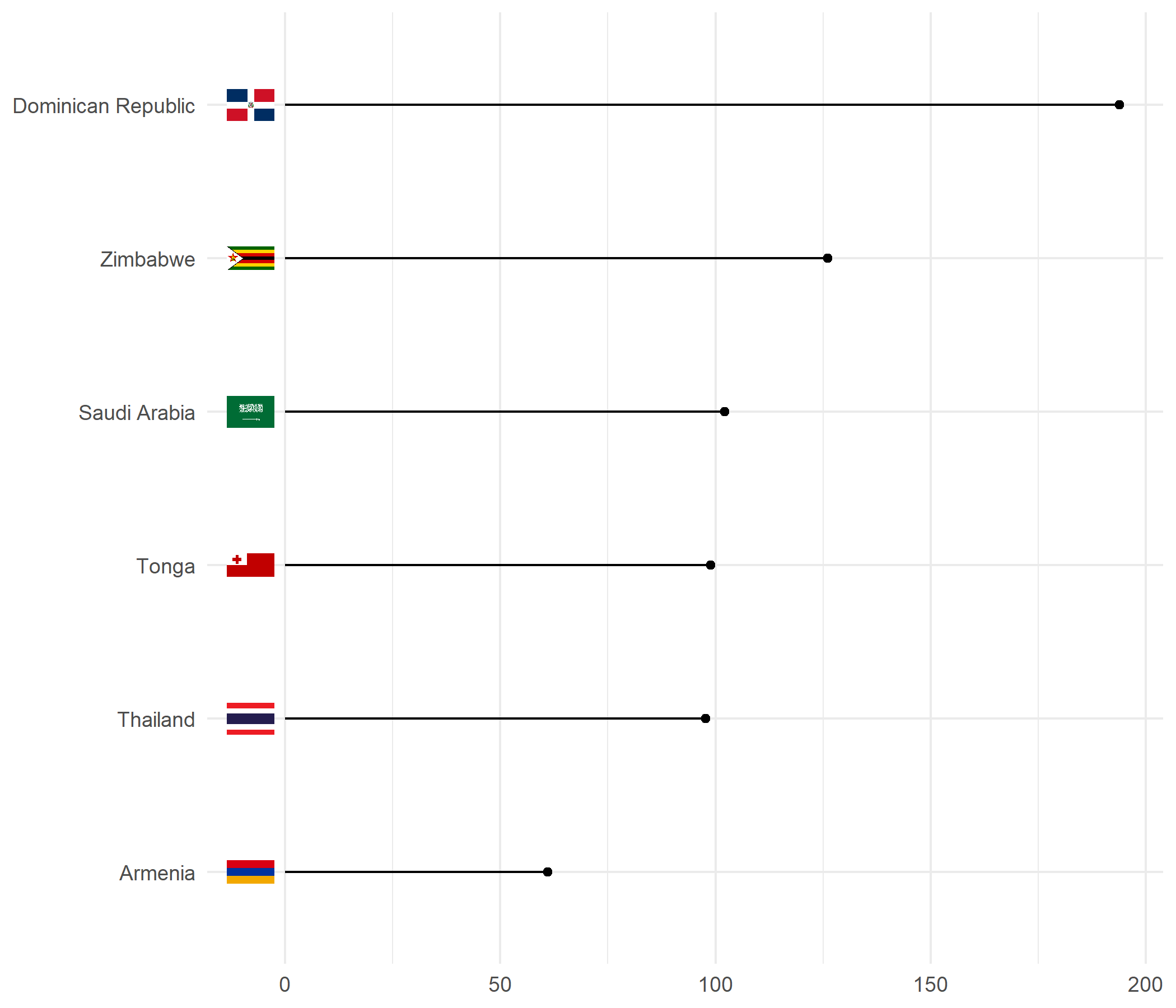
ggimage_part1 + labs( title = paste( "Countries with the highest road", "traffic death rate (per 100k", "population) \nwithin each", "continent" ) )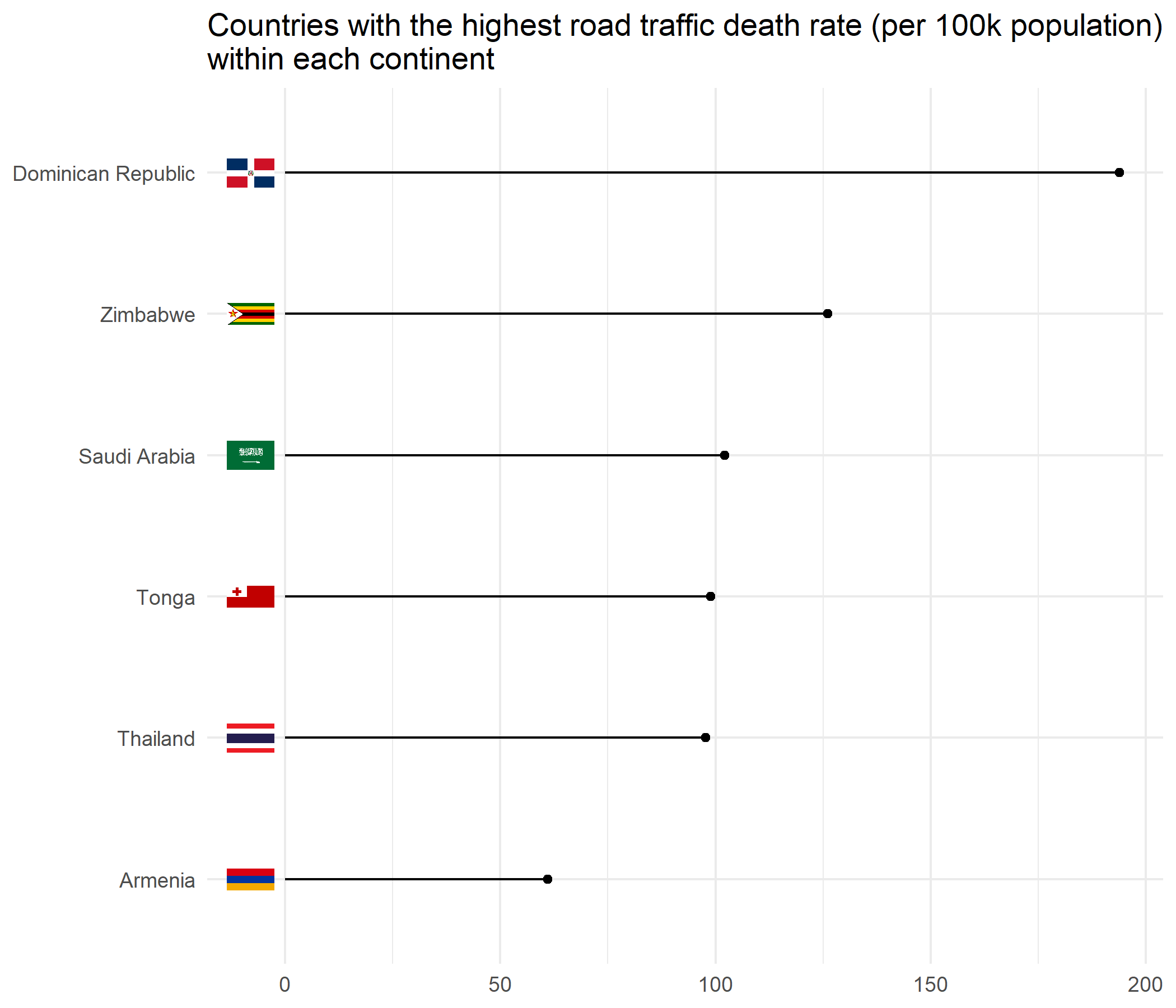
ggimage_part1 + labs( title = paste( "Countries with the highest road", "traffic death rate (per 100k", "population) \nwithin each", "continent" ) ) + labs(caption = "Data source: WHO")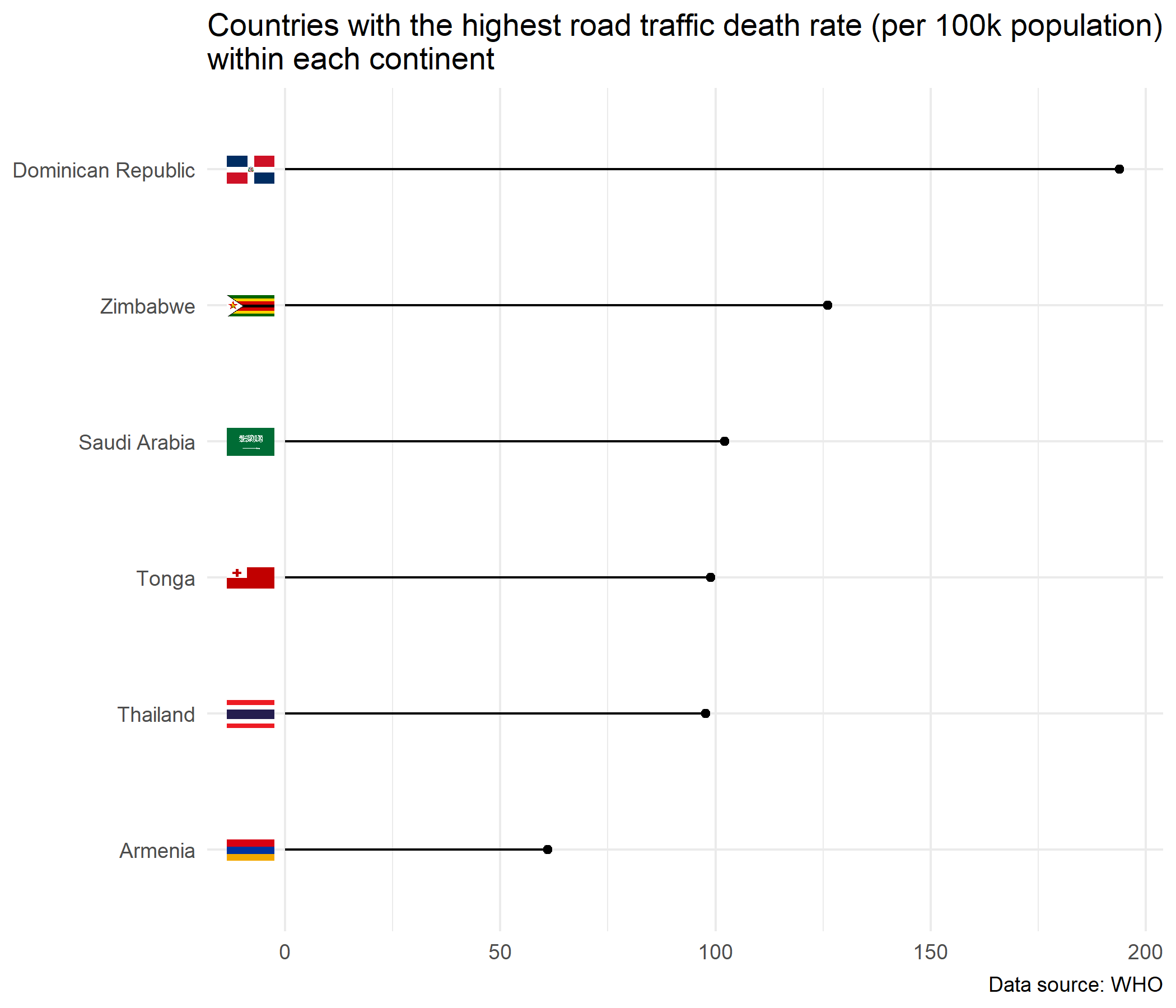
lol_chart + labs( title = paste( "Traffic crash death rate", "per midwest state, 2018" ) ) + theme_bw()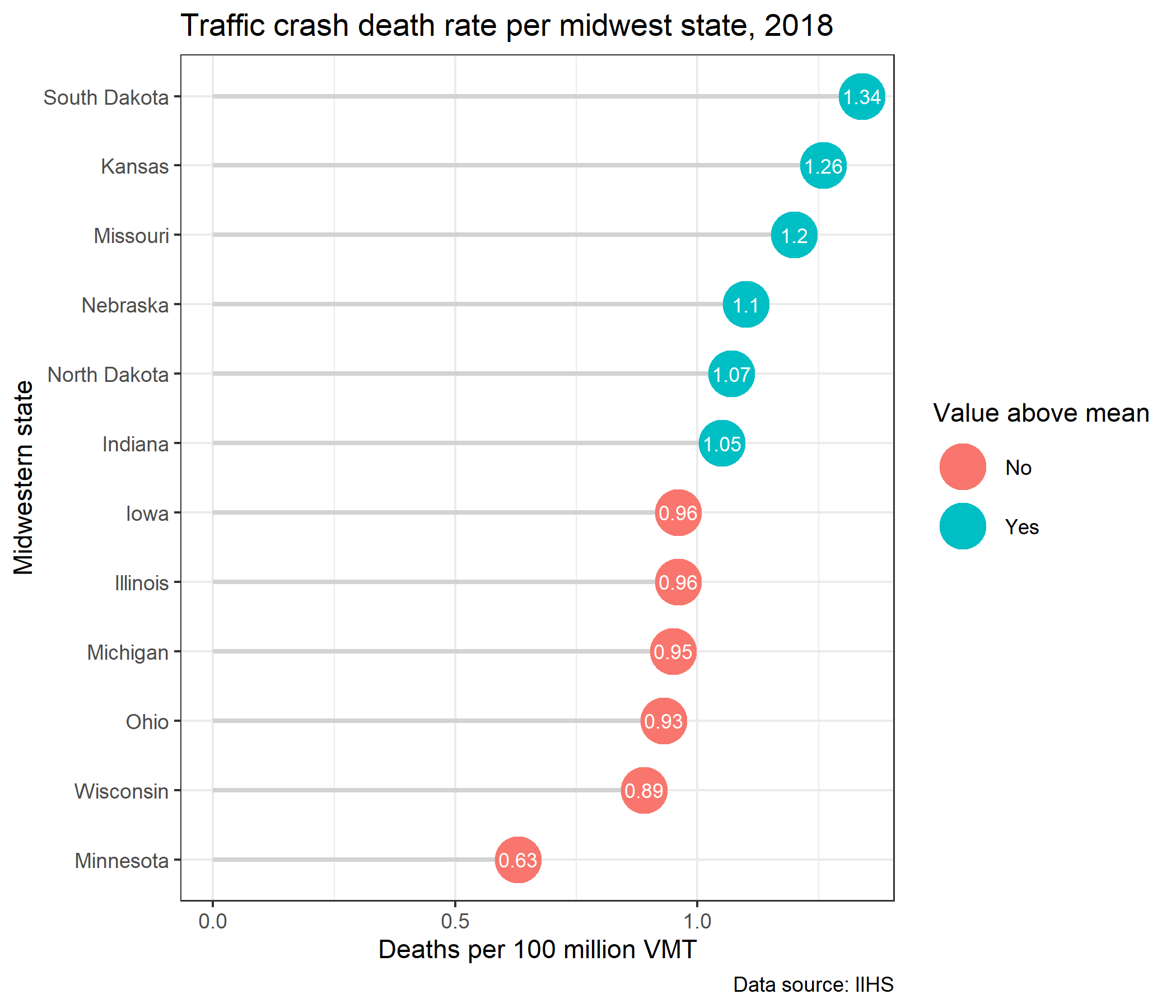
lol_chart + labs( title = paste( "Traffic crash death rate", "per midwest state, 2018" ) ) + theme_solarized()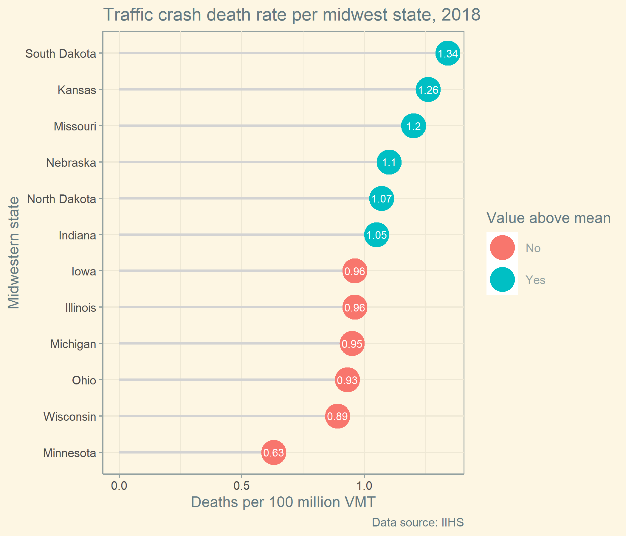
lol_chart + labs( title = paste( "Traffic crash death rate", "per midwest state, 2018" ) ) + theme_fivethirtyeight()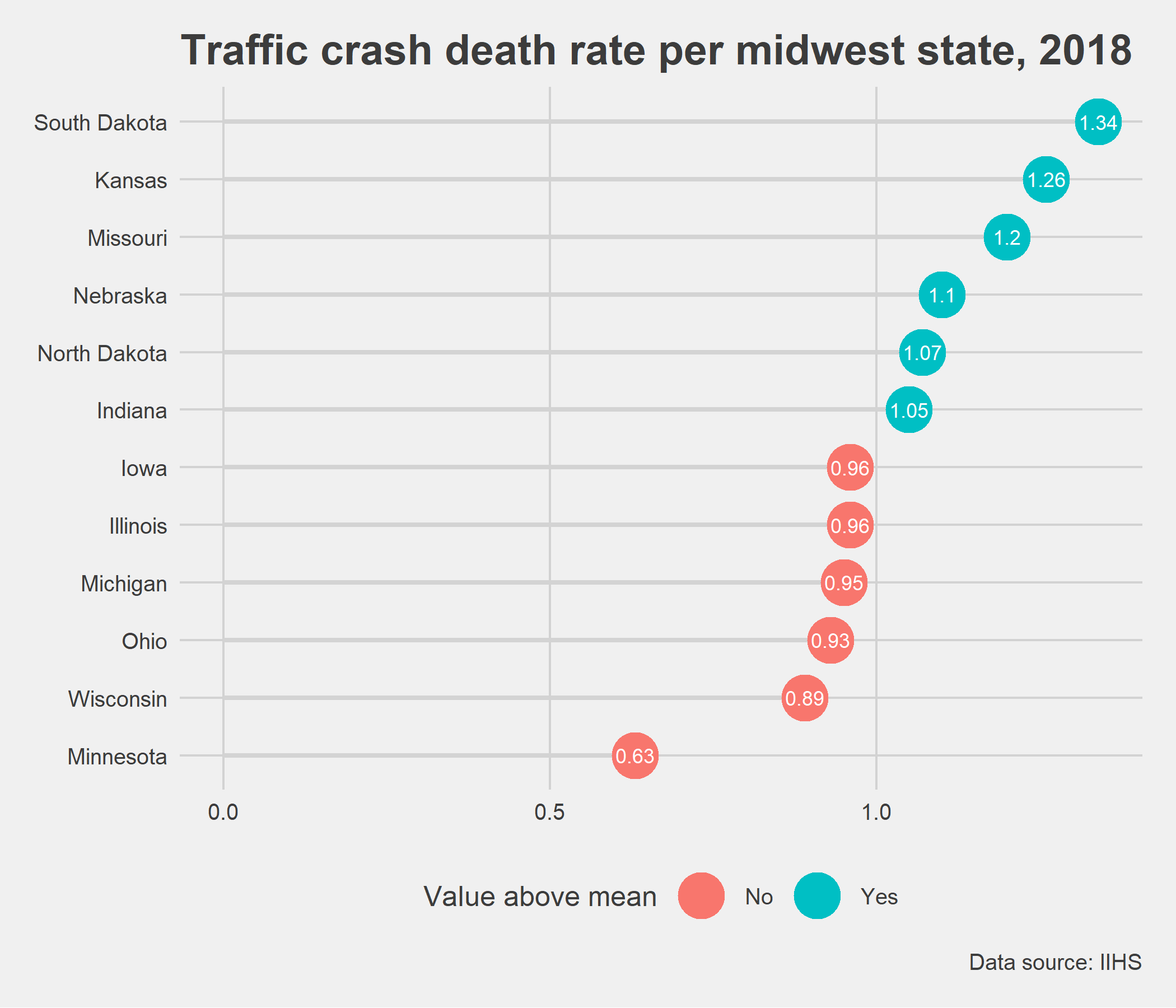
lol_chart + labs( title = paste( "Traffic crash death rate", "per midwest state, 2018" ) ) + dark_mode(theme_fivethirtyeight())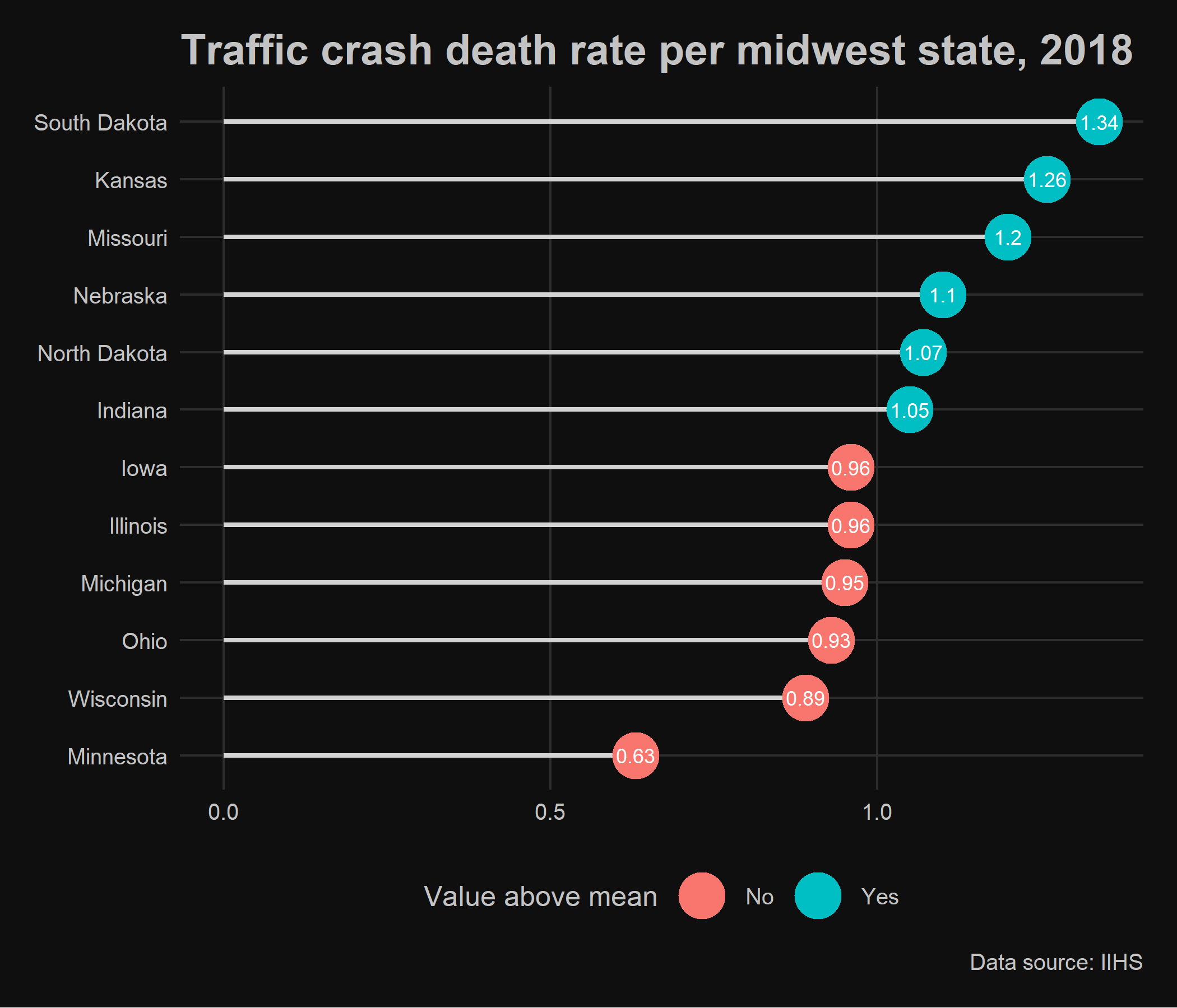
lol_chart + labs( title = paste( "Traffic crash death rate", "per midwest state, 2018" ) ) + theme_economist()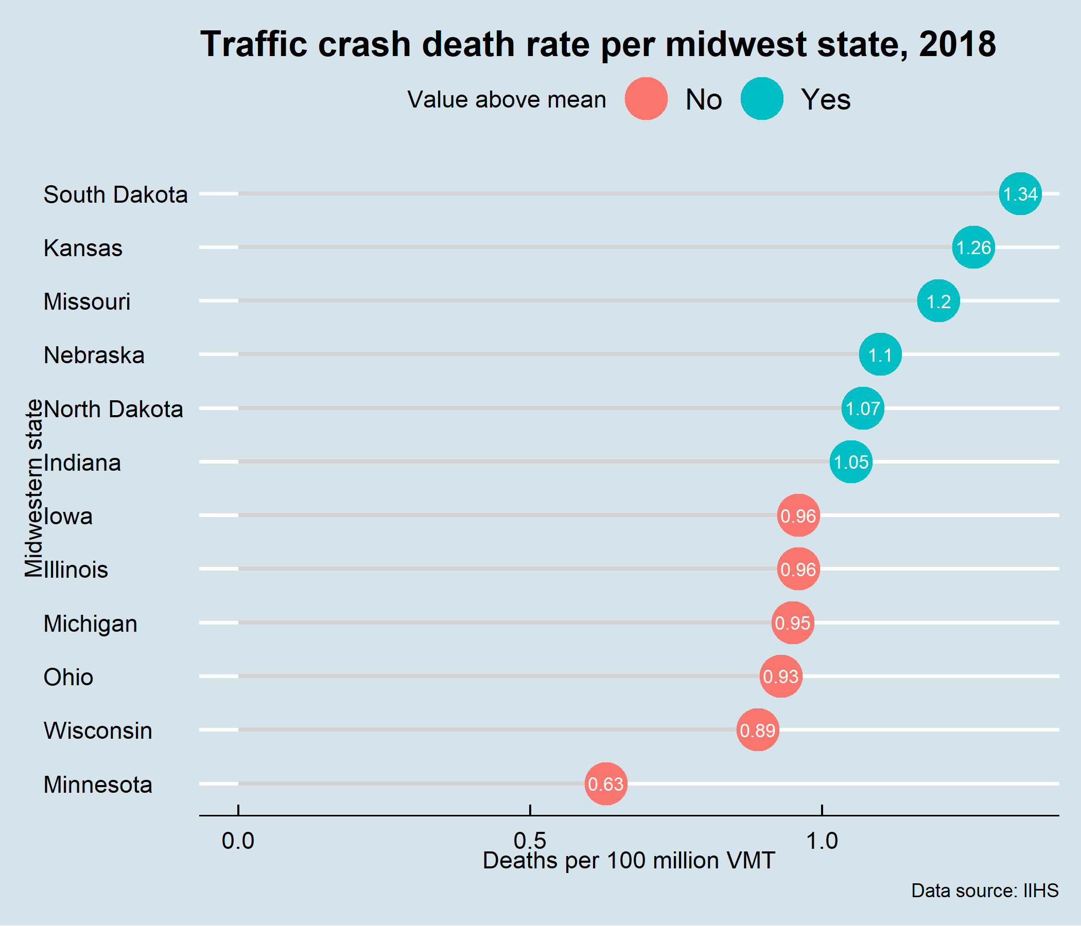
lol_chart + labs( title = paste( "Traffic crash death rate", "per midwest state, 2018" ) ) + dark_mode(theme_economist())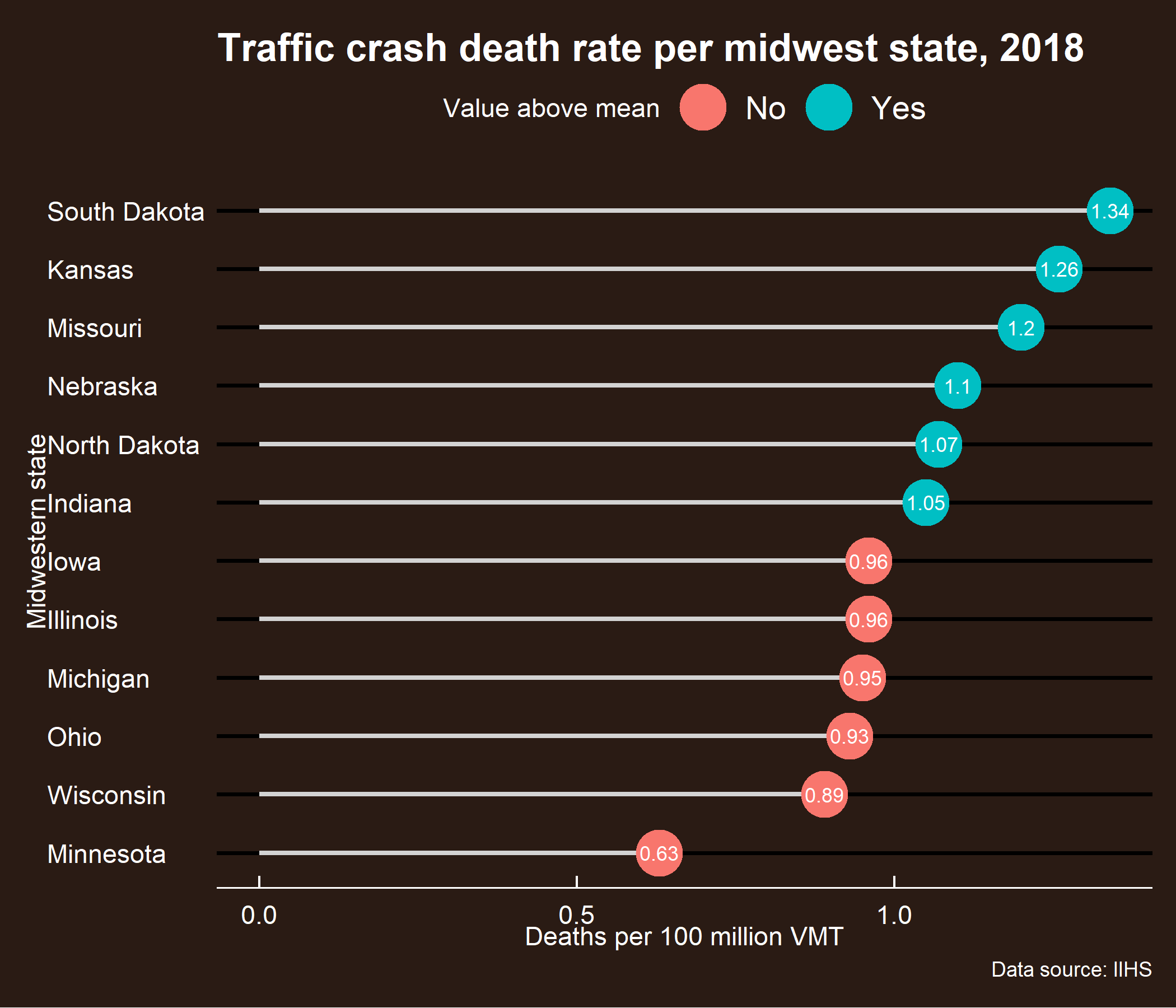
lol_chart + labs( title = paste( "Traffic crash death rate", "per midwest state, 2018" ) ) + theme_economist_white()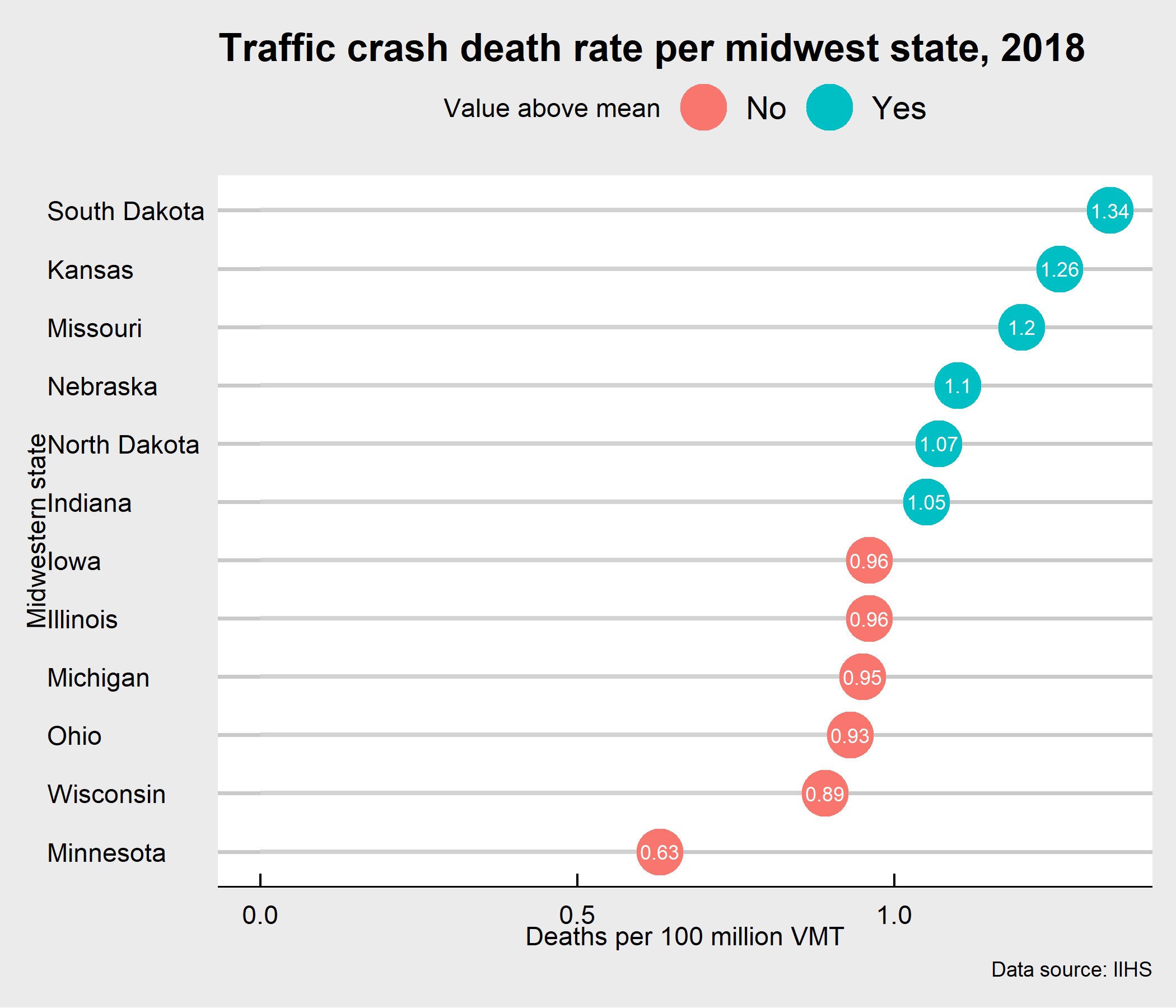
Closing remarks...

(Available at [http://gph.is/2porEcP](http://gph.is/2porEcP), Mar 14, 2021)